Introduction to Paraview

Overview

Teaching: 15 min
Exercises: 0 min

Questions

• What is Paraview?

Objectives

• Understand what Paraview is and where it can be used.

Paraview and Visualization

Paraview is an open-source science/data visualization and data analysis package developed by Kitware, that is designed for interactive and batch use within many domains and disciplines, such as engineering, computational fluid dynamics, medical science, material science and sensor data.

But what is visualization? Visualization is a powerful tool for displaying at complex, multi-dimensional data in a way that is easier to understand. Below are some examples.

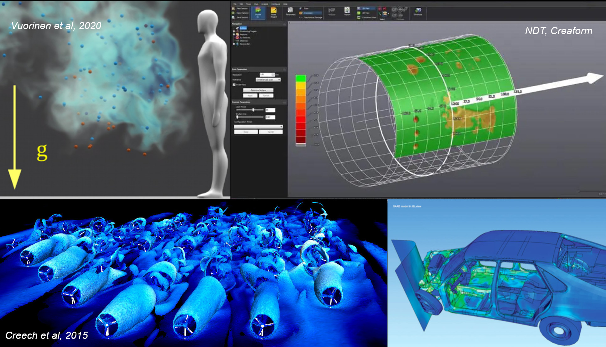
Paraview is capable of doing visualizations like you can see above - in fact, it was used to produce some of them. With practice, you can too. This lesson will help you get to grips with the basics of Paraview, and set you on the road to creating your own visualiations.

How Paraview can be run

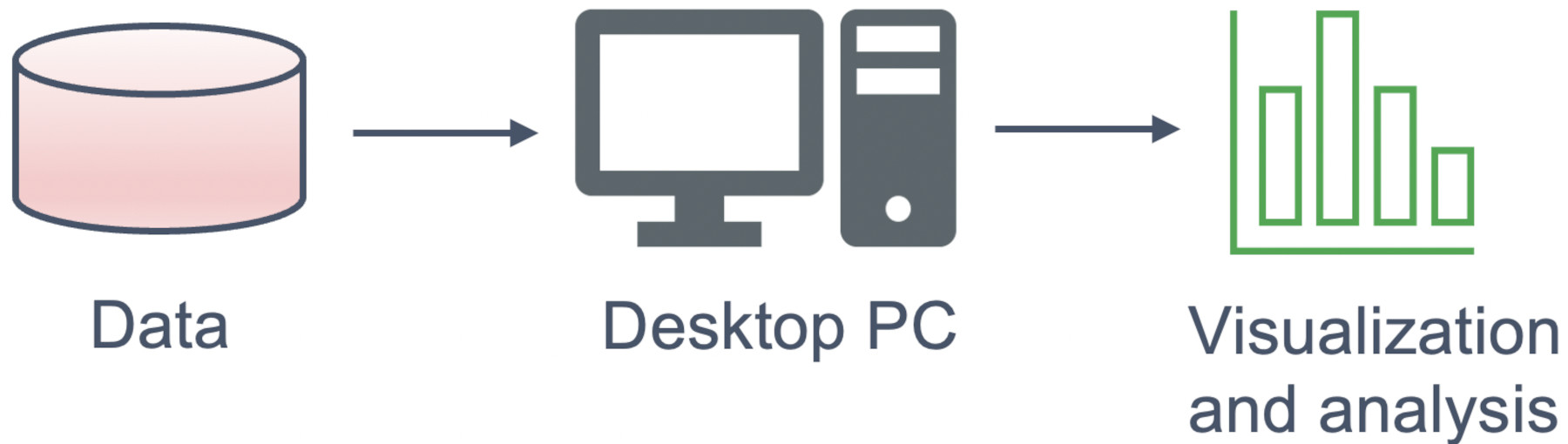
Paraview can be run straight from a desktop, reading data in directly from storage:

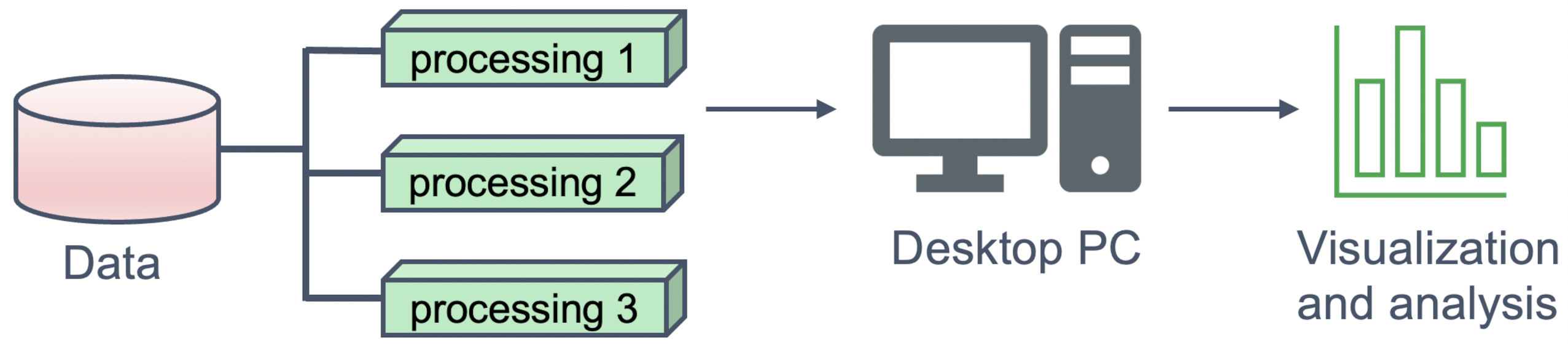
Alternatively, for very large datasets, Paraview can be run in client-server mode, with processing done remotely on a cluster or more powerful server computer, but rendered on a local desktop:

Processing data with filters

One of the most powerful features in Paraview, is that it can chain together a series of operations known as filters to operate on data. Filters can be connected in series, taking input from the previous filter’s output, operate on it, and pass it to the next filter.

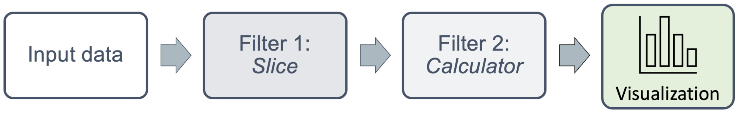
You can also `branch off’ the chain, with seperate filters to create multiple visualizations.

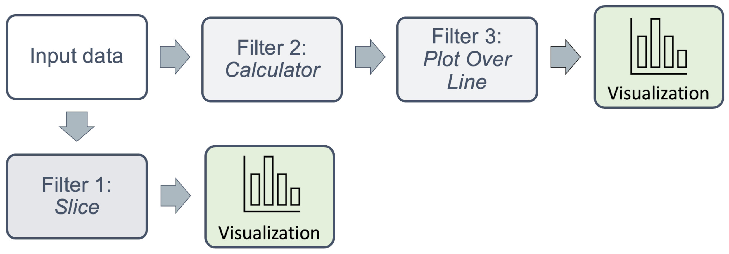
Each visualization appears in a seperate window frame within Paraview. What is particularly powerful, is that data from each can also be operated on, or saved individually to disc for further processing, eg. by a seperate application such as MatLab or a Python program.

Sources

Sources in Paraview are sources of data, which can be operated on by filters. This can be a file, or any item in the Sources menu, such as text, shapes, point or line sources. Some filters can combine sources together. This can be particularly useful in when restructuring data onto different grids, for example.

A few examples of types of data that Paraview can use are shown below.

Structured grids

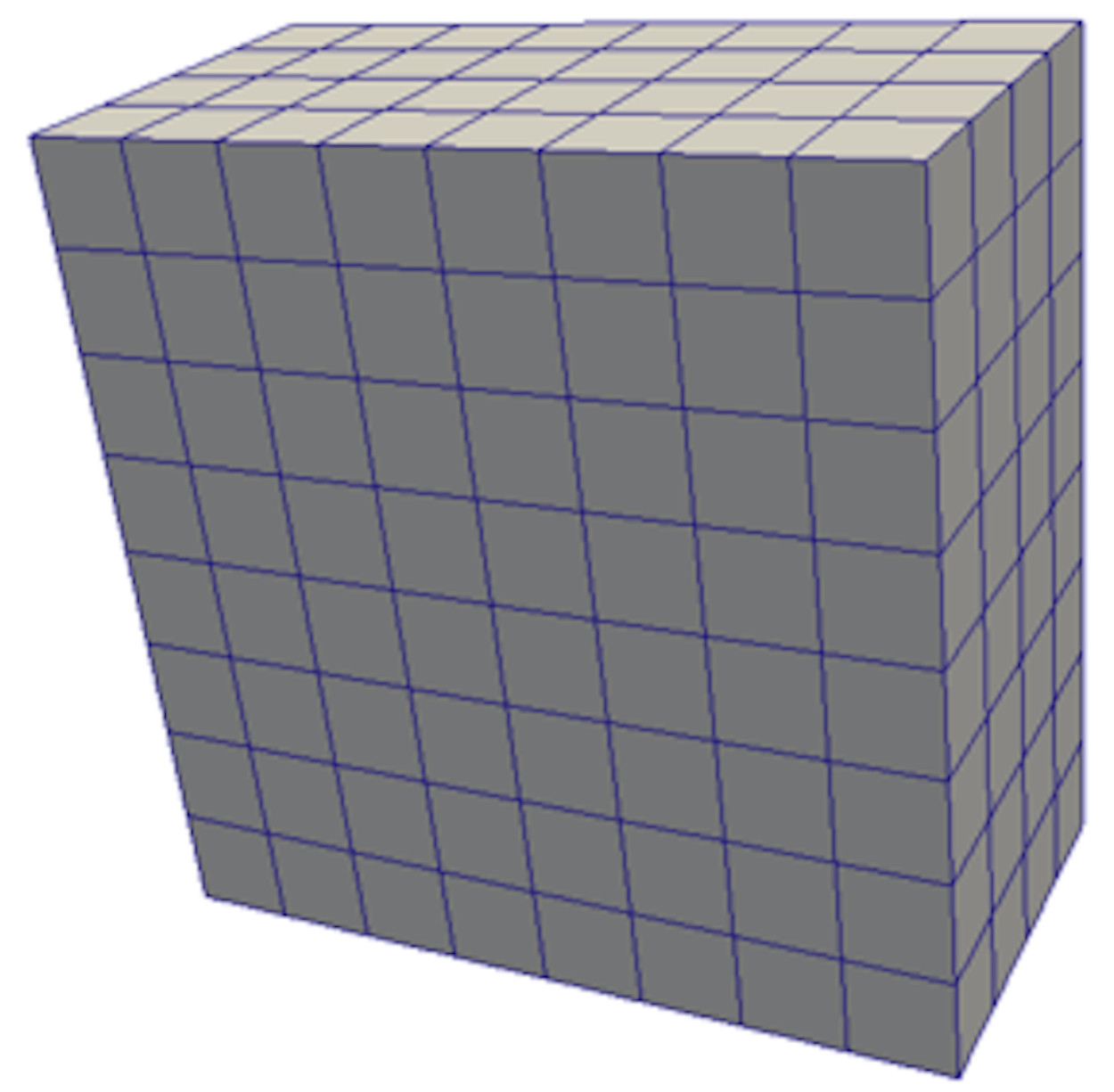
Structured grids have a regular, specified structure. Grid cells can be evenly spaced along the Cartesian axes, as is the case with the rectilinear uniform grid shown below.

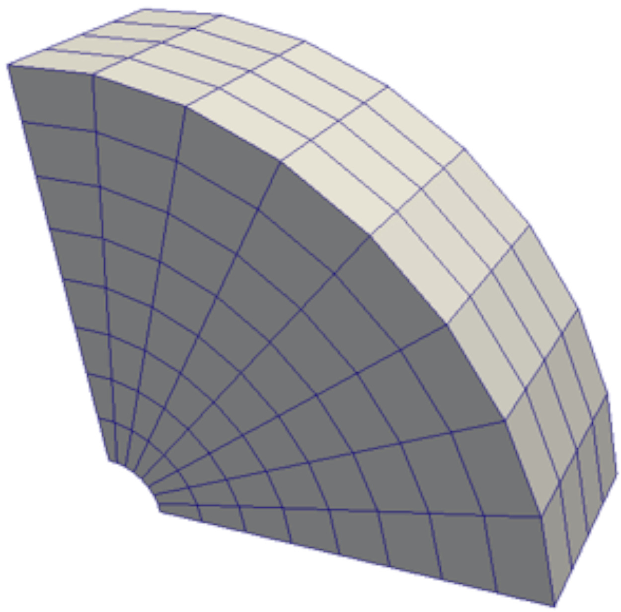
Or fitted using a cylindrical coordinate, as shown with the curvilinear structured grid below. Such a grid would typically be used to model a regular, tubular domain (eg. flow through a pipe).

Unstructured grids

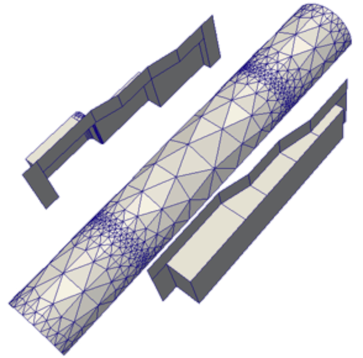
Unstructured grids have an arbitrary structure, which is completely dependent upon the meshing tool used to generate the mesh. They can be made up of arbitrarily-sized simplex shapes, eg. triangles, tetrahedra, hexahedra, or can be a mixture of multiple types, as shown here.

Paraview can operate on all 2D, 3D meshes without difficulty. The same types of processing can be applied to both structured and unstructured meshes, as long as the file format is supported.

Where to use Paraview

Paraview can be used in a variety of scientific, engineering and medical scenarios. There are covered in ACENET’s presentation High Performance Computing and Visualization: An Overview, which we will briefly recap here.

Key Points

• Paraview is open-source visualization software

• It loads in structured and unstructured 3D datasets of scalar and vector data.

• It is available for Windows, MacOS and Linux

Opening Paraview and viewing a dataset

Overview

Teaching: 15 min
Exercises: 5 min

Questions

• How do I look at data?

Objectives

• Understanding the window layout of Paraview

• How to open data and manipulate the view

Before you start

Paraview can be extremely demanding of your computer’s memory, especially on large data sets.

Please close down any unnecessary any unnecessary programs such as additional browser windows/tabs and office software before proceeding. If you do not, Paraview may run very slowly.

Opening Paraview

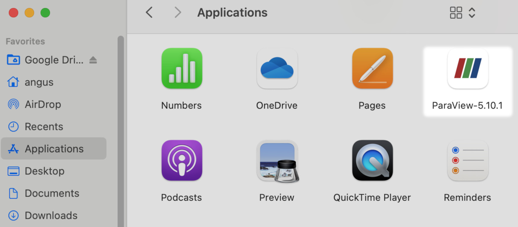
We’ll start by opening Paraview. Assuming you have installed Paraview, click on the Paraview icon. On MacOS, this will be in the Applications folder, ie.

Once started, you should see the Paraview application Window:

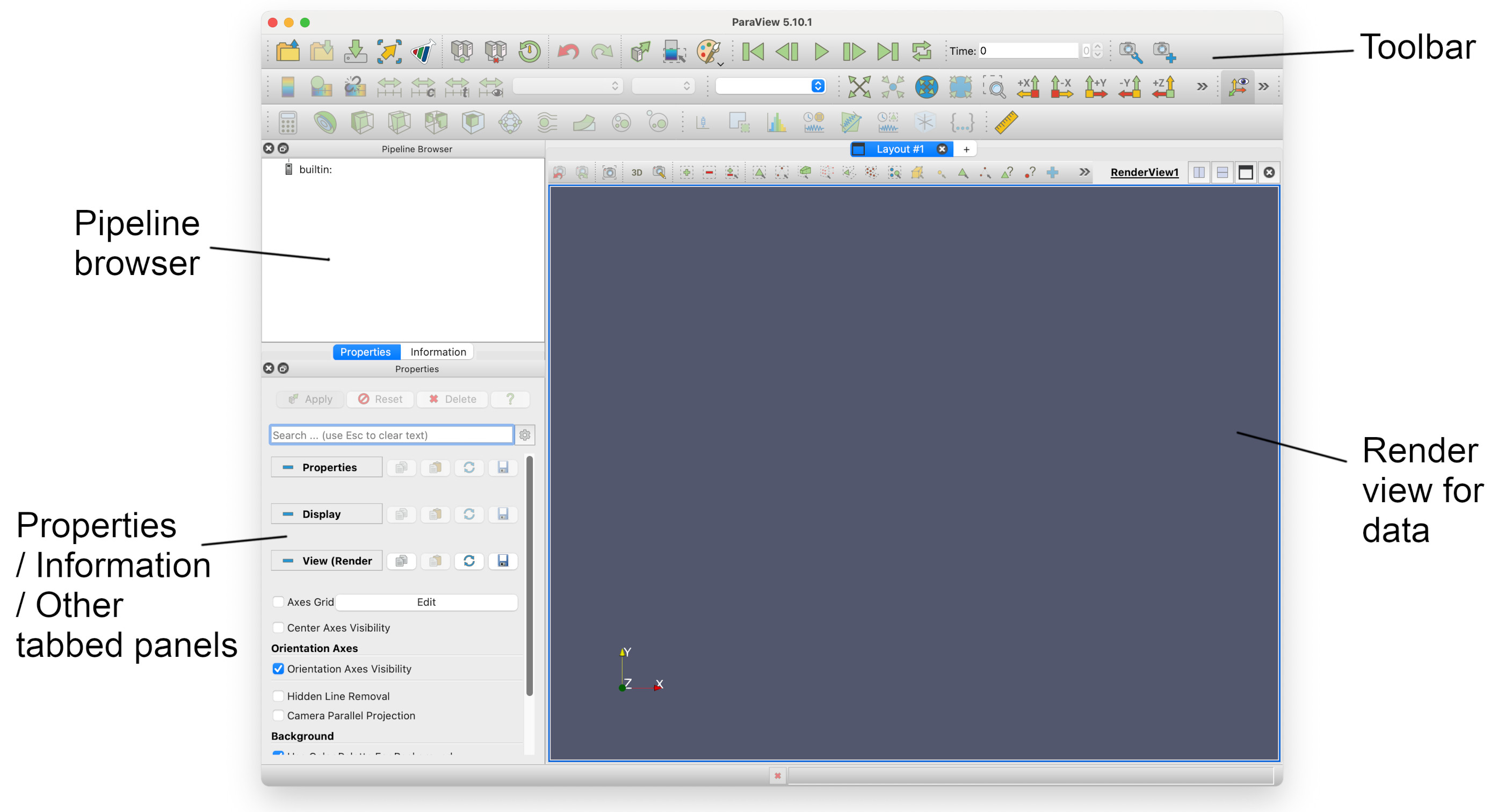
The four main sections of the application window are highlighed above.

The pipeline browser

This displays the processing pipeline in a tree view. Each data source will be a `root’, with filters as seperate or connected branches. It is interactive, allowing you to hide or show the results of filters. You can also select any item on the tree and display its properties.

Tabbed panels

This panel has two tabs, Properties and Information, although more can be added. These are active for the selected item in the Pipeline browser. Properties allows certain basic properties of the current view displayed in the Render view to be changed; Information displays details about the current view, such as number of points, cells and bounds.

The render view

This displays the rendered output produced by the sources and filters in the Pipeline browser. Here you can manipulate the view using the mouse.

The toolbar

The toolbar contains icons which for a selected subgroup of actions and submenus. These are grouped together into file functions, animation functions, field options, view options, and filters. Depending on what part of the pipeline is selected, some of these may be disabled and grayed out.

NB. The complete list of options and commands in MacOS are in the drop-down menus at thetop of the screen (not shown). Under Linux and Windows, these are at the top of the main Paraview window, above the toolbar.

Opening a file

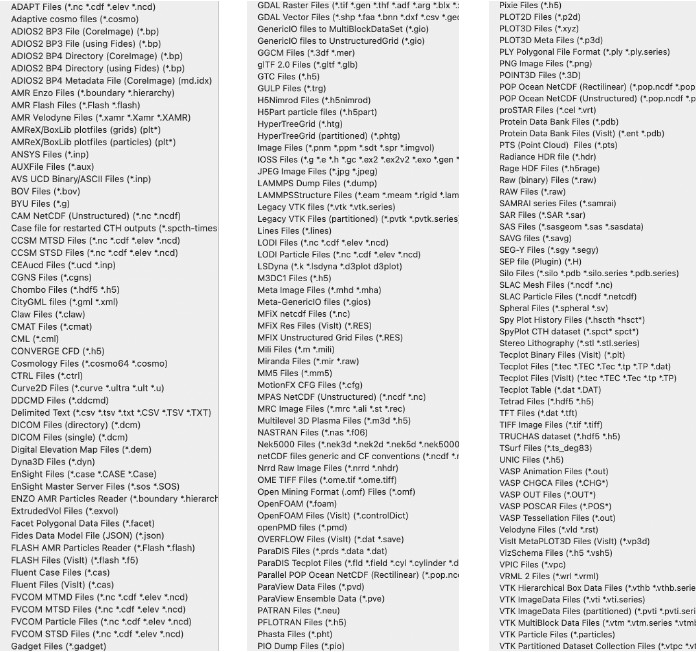
Paraview can import many types of data file formats. Here’s a non-exhaustive list:

We are going to open one of the tutorial data files that you have unarchived onto your desktop. If we click on the *open file* icon 

We get to the open file dialogue -

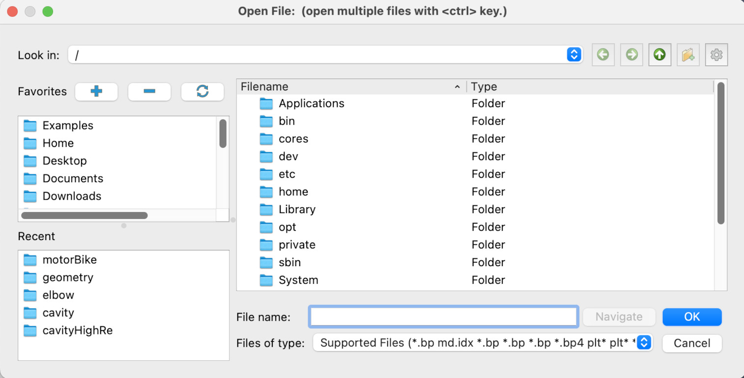
Click on Desktop, then acenet-paraview-tutorial, then disk_out_ref.ex2. Click the Apply button, and you should now have a view similar to this.

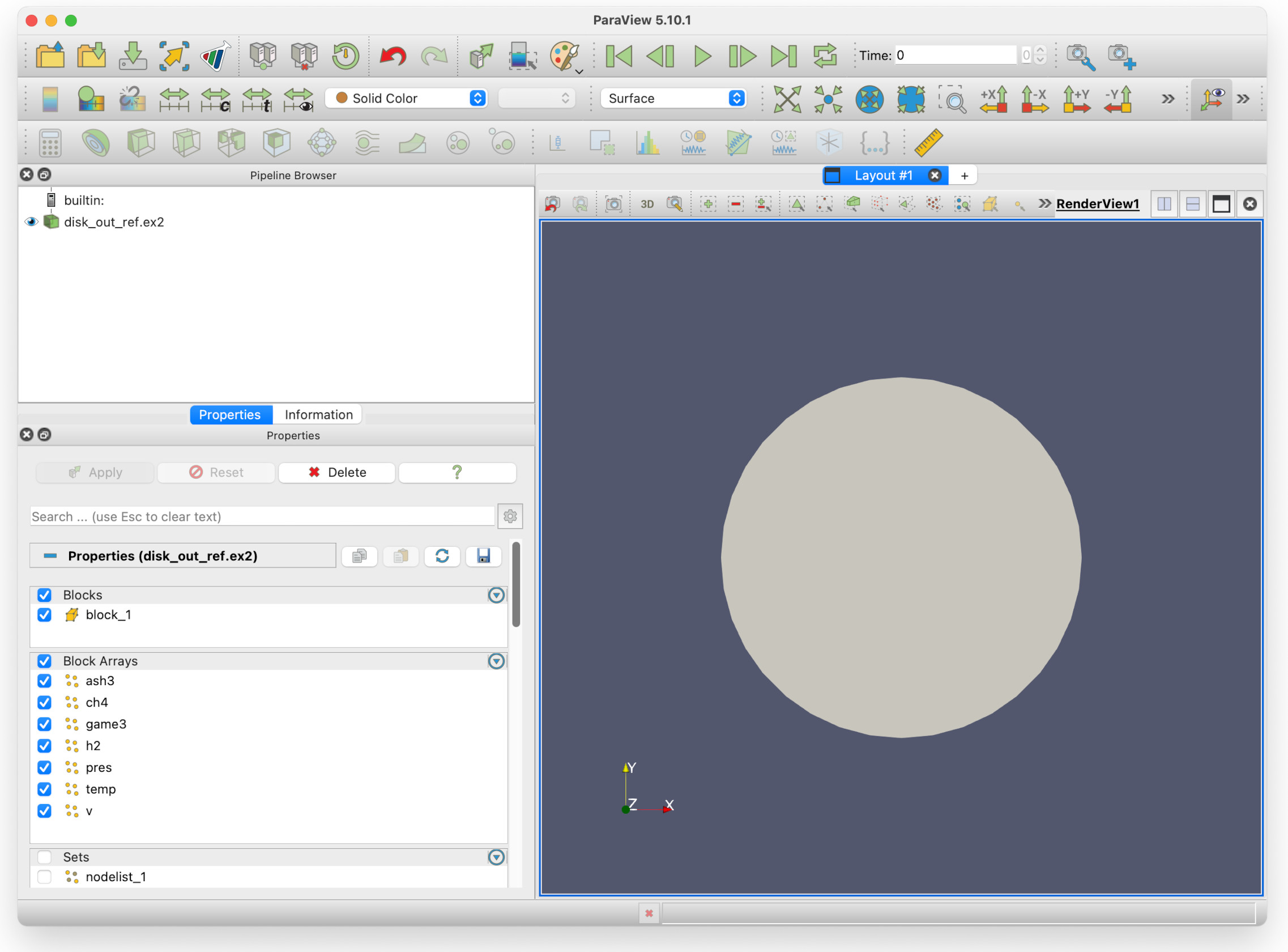
Information about the data file

You can see in the Pipeline browser that there is one data source: disk_out_ref.ex2, the file that has been loaded in. The eye icon beside it can be clicked, to show/hide the view.

The Properties panel shows you the Blocks available (block_1), and Block Arrays shows you the data fields available. The check marks beside them indicate they are enabled for processing.

In the Sets sub-pane (you may need to scroll down with the mouse wheel) there are nodes and surface lists. If we deselect the block in Block Arrays we can select individual surfaces we would like to view.

Manipulating the view

The first thing we can try is colour the object with a data field. In the tool bar, you will see a drop-down box that current contains Solid Color. There is a second menu to the right, labelled Surface. This is the current representation of the object. This can be changed to Points, Surface with edges, Volume, etc. if you so wish.

Click on it and select v (for velocity). This colour the cylinder and also add a legend on the bottom right indicating the range of values within the field.

You can experiment with rotating and changing the view. There are several mouse actions you can use to do this:

• Left click and drag will rotate the data view about the origin.

• Scrolling the mouse wheel will allow you to zoom in and out.

• Middle click and drag will move the object around the render view window.

Try rotating the view so you can see hole in the cylinder.

Key Points

• Paraview supports many types of formats

• It can view 2- and 3-dimensional data

• The mouse can be used change the view

Introducing filters

Overview

Teaching: 20 min
Exercises: 10 min

Questions

• How do I filter data?

• Can I show multiple views?

Objectives

• Attaching a filter to an opened file

• Chaining filters together

• Changing the order of filters

Overview of filters

A filter is a processing unit that takes data from a data source or other files, and produces output. Filters can be chained together, typically with the last in the chain shown. Filters can be branched off too, so one data source can have multiple filters independently operating on its data.

There are a great many filters available. Paraview categorises them in the Filters menu so you can find what you want easier.

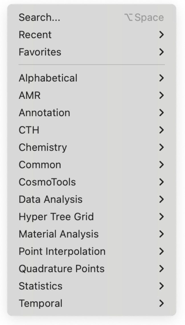
We will mostly dealing with those in the Common submenu.

Adding the first filter

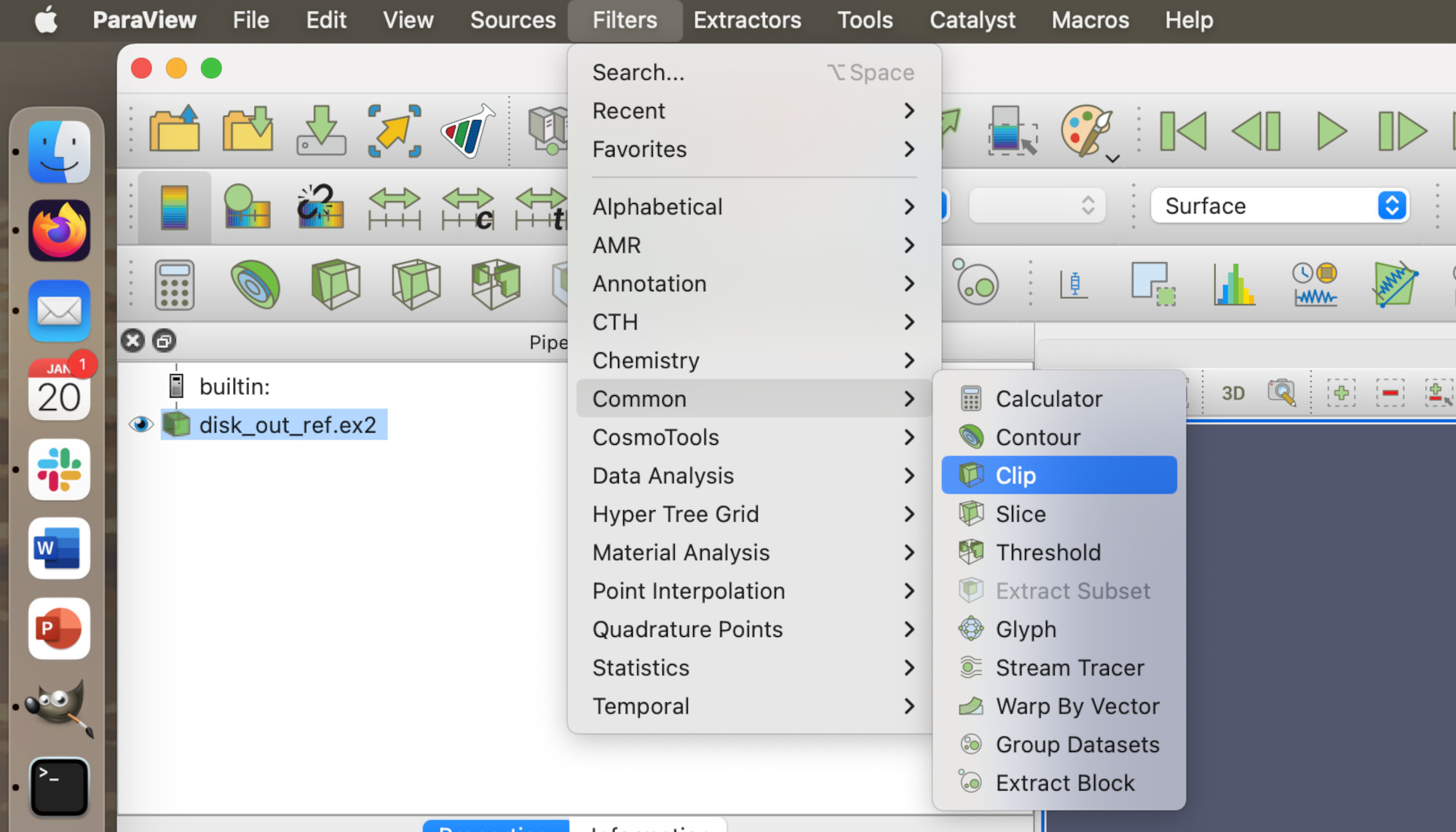
We will start from where we left off in the previous lesson. Here, we are going to apply a filter to see is happening to the gas inside the chamber. We are going to do this by applying the Clip filter.

First, click on disk_out_ref.ex2 in the Pipeline browser and then go into the Common submenu in the filters, select the Clip filter.

Click Apply. You should now see a render view similar to this.

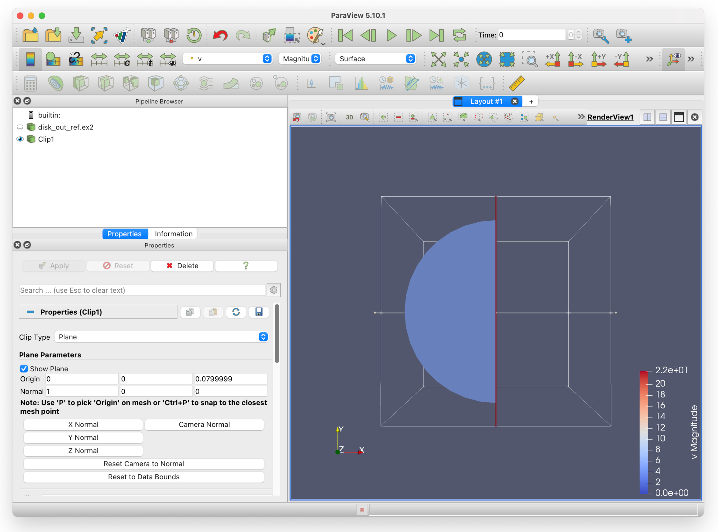
Note that in the Pipeline browser, disk_out_ref.ex2 has a greyed-out eye icon next to it, and Clip1 - our clip filter - has a solid black eye icon. This is to indicate that the view of disk_out_ref.ex2 is hidden from view. If you show wish to see it again, you can click the faded icon to show it - however, this will obscure the Clip1 view.

Next, we will rotate the view so we can see the fluid velocity within the chamber. You can do this in one of two ways:

1. Rotate the view with Left mouse click and drag as shown previously, or
2. Hit the -X rotation button in the toolbar.

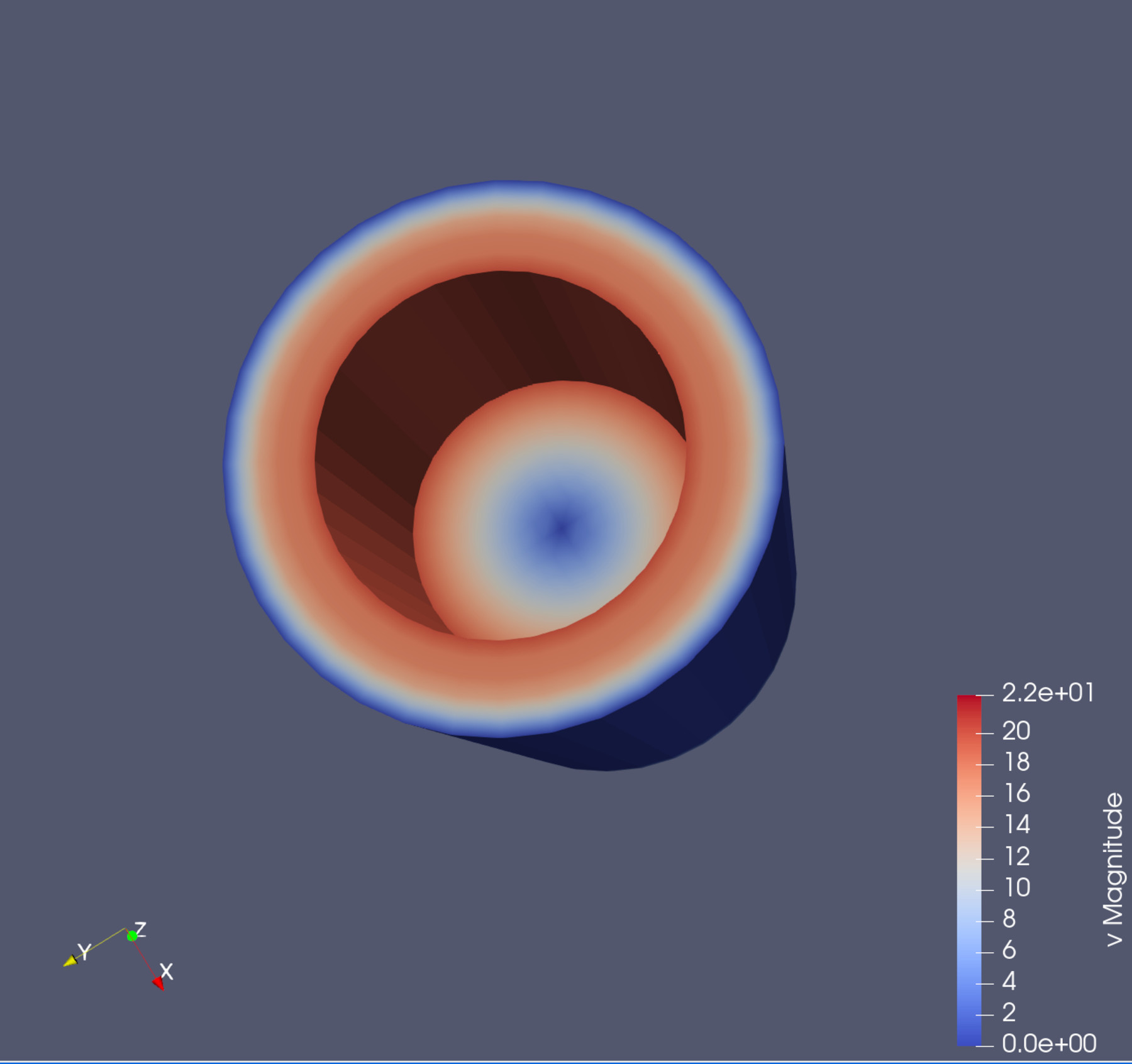
Which should give you this:

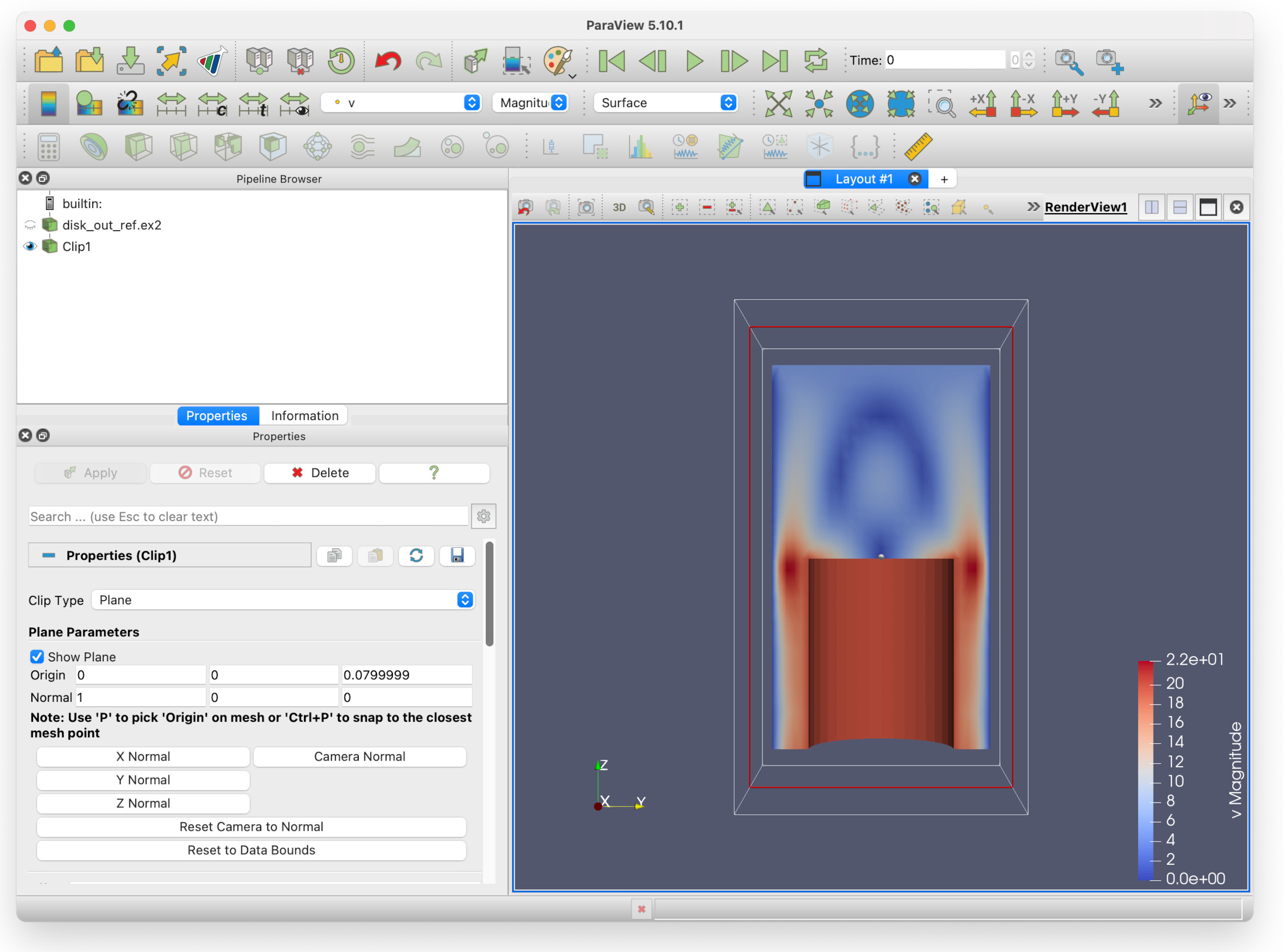
You can see that fluid speeds up and moves around the sides of the piston, which is what we would expect as it moves up and down. By looking at this picture, the physics of the situation can be clearly understood by a non-expert. This shows one of the many strengths of visualisation.

But what is happening to the pressure? How would we show that? Can we show it alongside the velocity?

Multiple filters and multiple views

Here we are going to do two things:

1. Create a second filter
2. Create a second render view to show the results of that filter

Creating a second filter

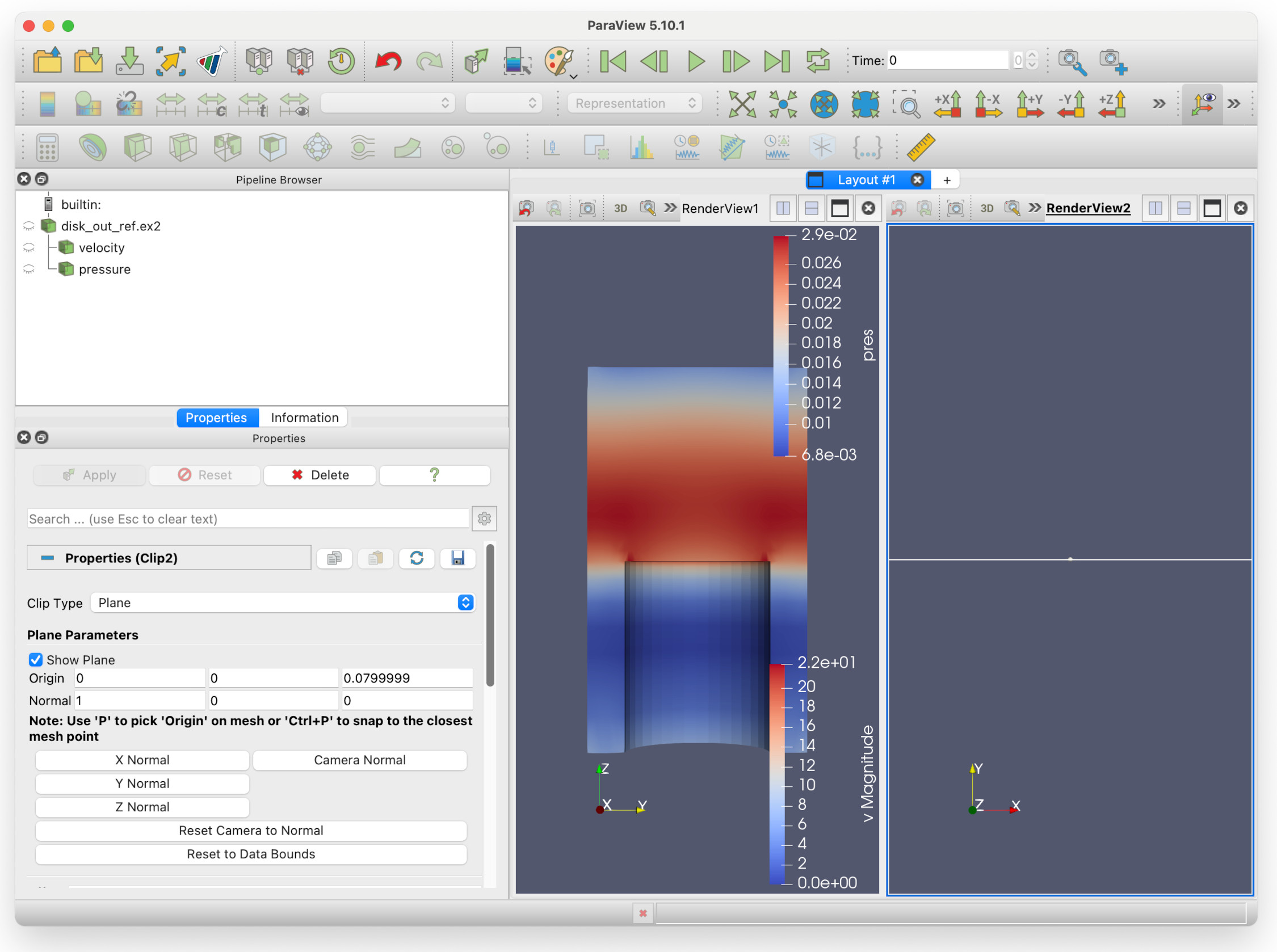
Go into the Filters/Common submenu and select Clip, then hit the Apply buttom. You will see the following view.

Notice that the colours have changed. This is because the view of the second clip (pressure) has obscured the first (velocity). This is what we are going to fix.

Firstly, Clip1 and Clip2 are ambiguous names. Let’s rename the filters so they cause less confusion.

• Right click on Clip1 and select Rename. Type `velocity’.
• Right click on Clip2 and select Rename. Type `pressure’.

Creating a second render view

Now we will create a second render view, in which we will show the pressure. This will allow us to look at both velocity and pressure of the fluid side-by-side.

To the right of the RenderView1 label at the top the render pane, click on the vertical split icon.

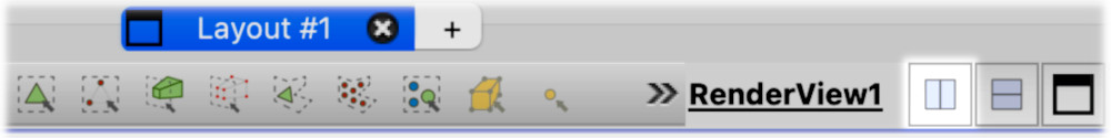
You will see a second pane that asks you to Create view. Select Render View. You will now have two render views in the layout / render view pane:

The second render view is empty: this is because both filters are displaying in RenderView1, none of them are in RenderView2. You can also see that all the eye icons in the Pipeline Browser are faded: this is because RenderView2 has been selected, but none of the filters are visible in that render view. If we click on the eye icon next to pressure, we should see that the pressure is now displayed in RenderView2, to the right of RenderView1.

A note of caution here - each render view has its own viewing angle, viewing distance and field selection, so we will have to go through the steps we did for RenderView1:

1. Press the -X axis button
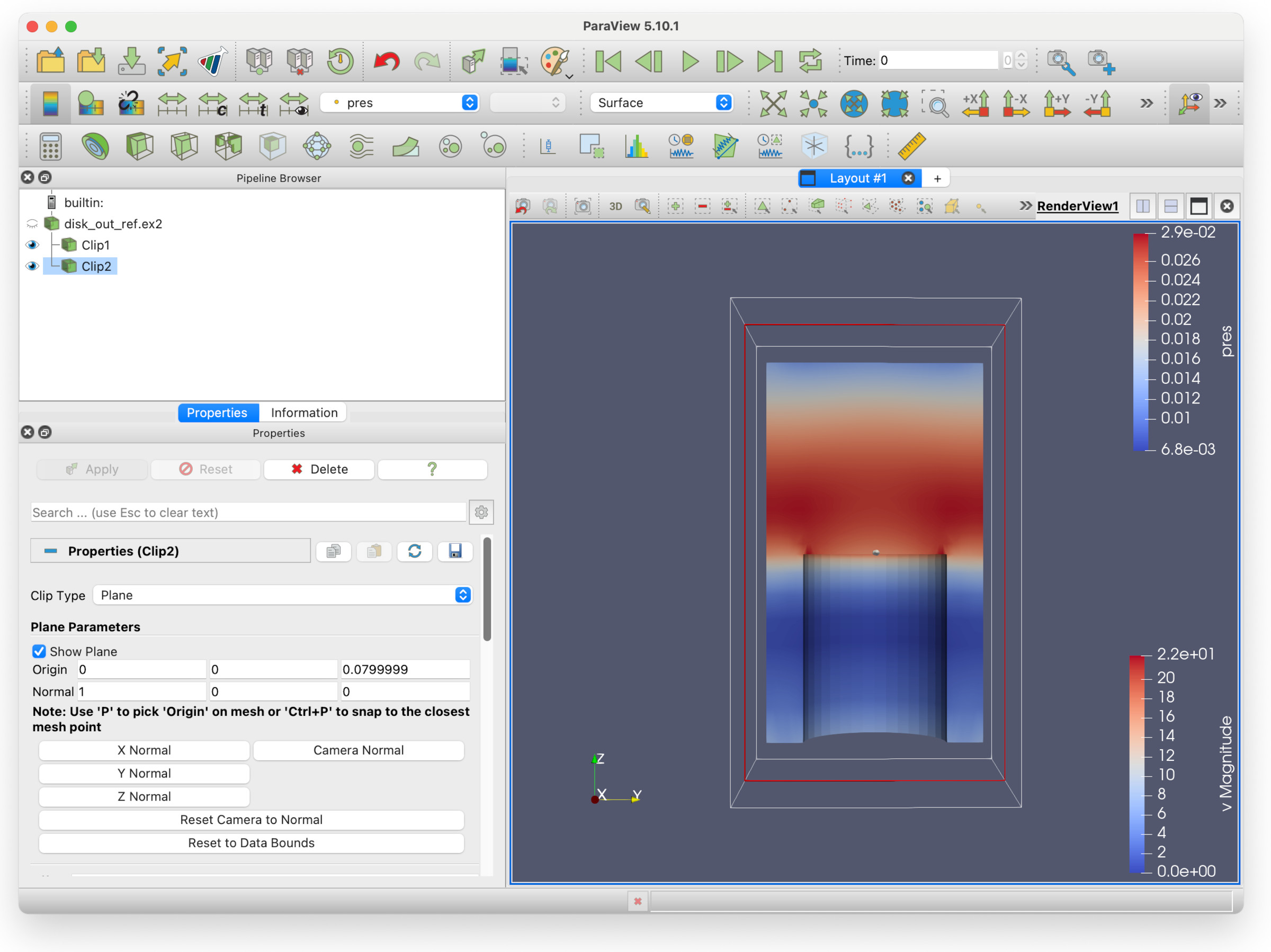
2. Change Solid Color in the colour selection toolbar menu to pres (pressure).
3. (Optional) Zoom to the cylinder with the mouse scroll wheel.

Which gives you this view:

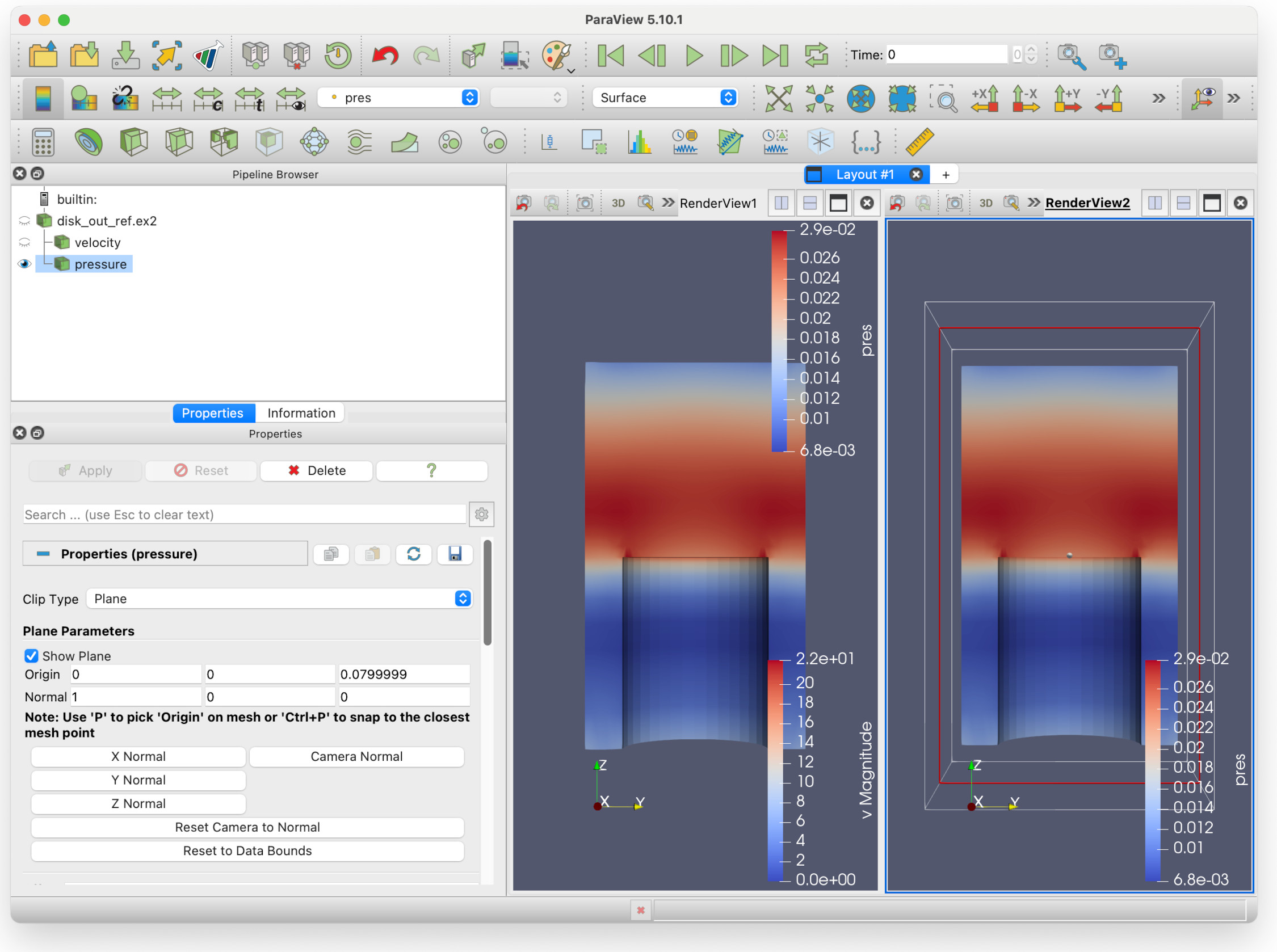
But hang on here - we are seeing two identical views of the pressure field! Surely something is wrong? No, not quite - this is just showing one of the key features of Paraview: multiple filters can be shown in multiple views at the same time, from different viewpoints if need be.

Remember we mentioned that we can select render views? Let’s try that now. Left click on empty space within RenderView1. There now be a thin dark blue rectangle around RenderView1 (which was previously around the second render view).

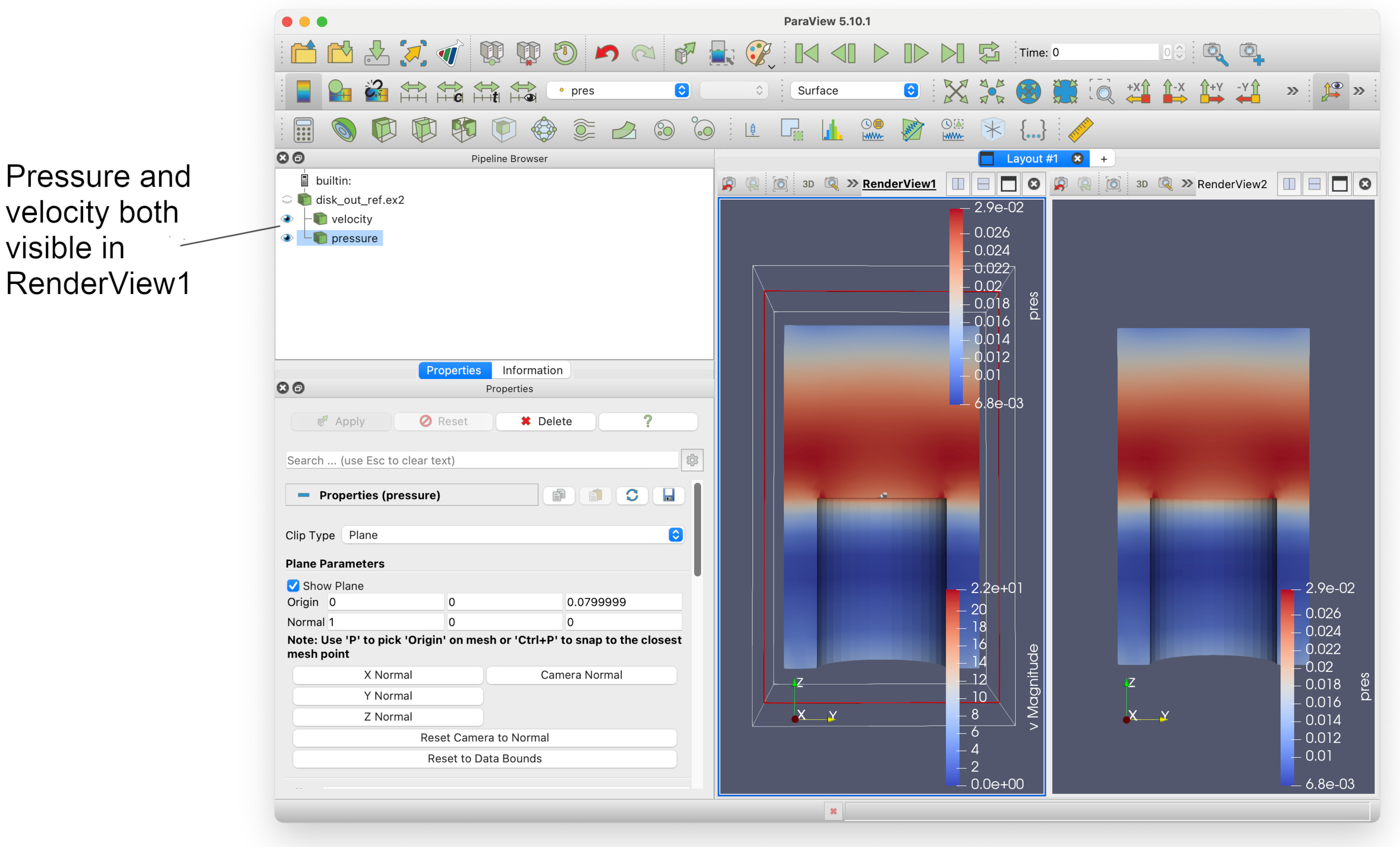
We can see that both velocity and pressure are visible in RenderView1. If we select the eye icon to the left of pressure, it should fade out. We can now have two render views, showing velocity and pressure side-by-side.

Changing the colourmap

Colourmaps (or colormaps!) tell Paraview how to colour the data according to the value. So if you have a temperature field with a colourmap defined to set be red at 30C, and blue at -30C, then warmer or colder temperatures will be coloured accordingly. Any values in between those ranges will have the colour interpolated between red and blue.

Colourmaps can be quite sophisticated, and you can even create your own. Paraview however has many good presets which you can use, and you may find giving different filters distinct colourmaps will make visualizations clearer. We will do that now.

1. Click on the left render view (RenderView1). 2. Select Clip1 in the Pipeline browser. 3. Select Properties in the tabbed panes on the left. 4. Scroll down until you see the folder with the heart icon, and click on it.

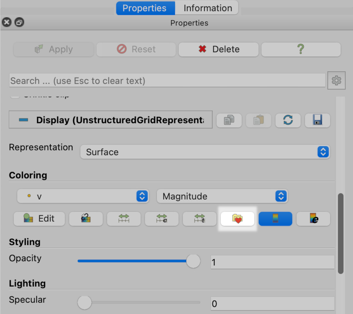
This will give you the colourmap dialogue:

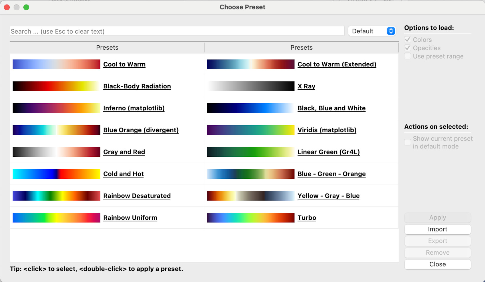
Here, the Rainbow Desaturated colourmap will be chosen, but of course you can pick any one. Note, the pull-down menu on the top-right where Default is currently selected. There are many, many more colourmaps available: if you select All instead of Default, the dialogue window will display every colourmap available.

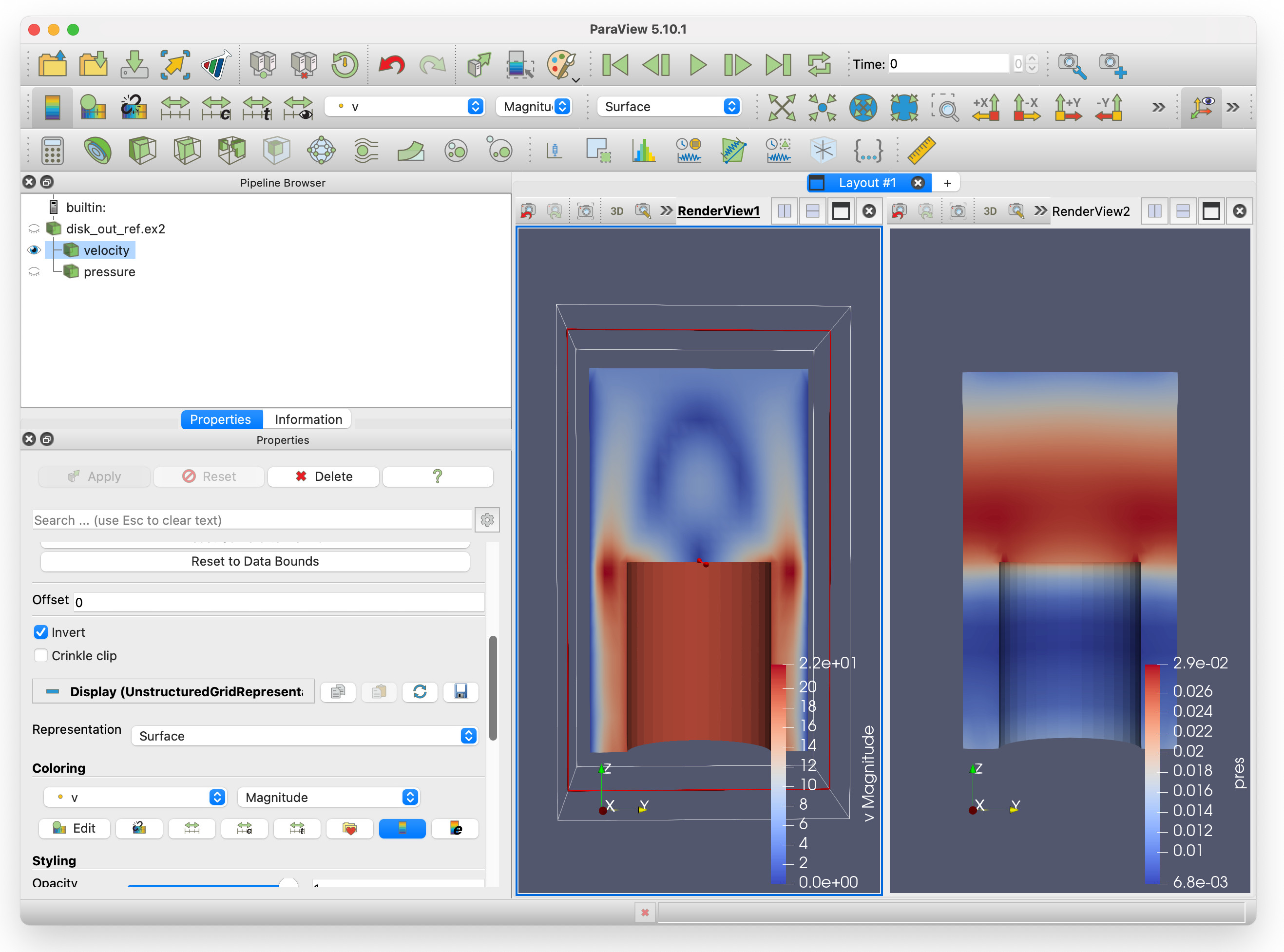
5. Once you have chosen a colourmap, click Apply then Close. { start=5 }

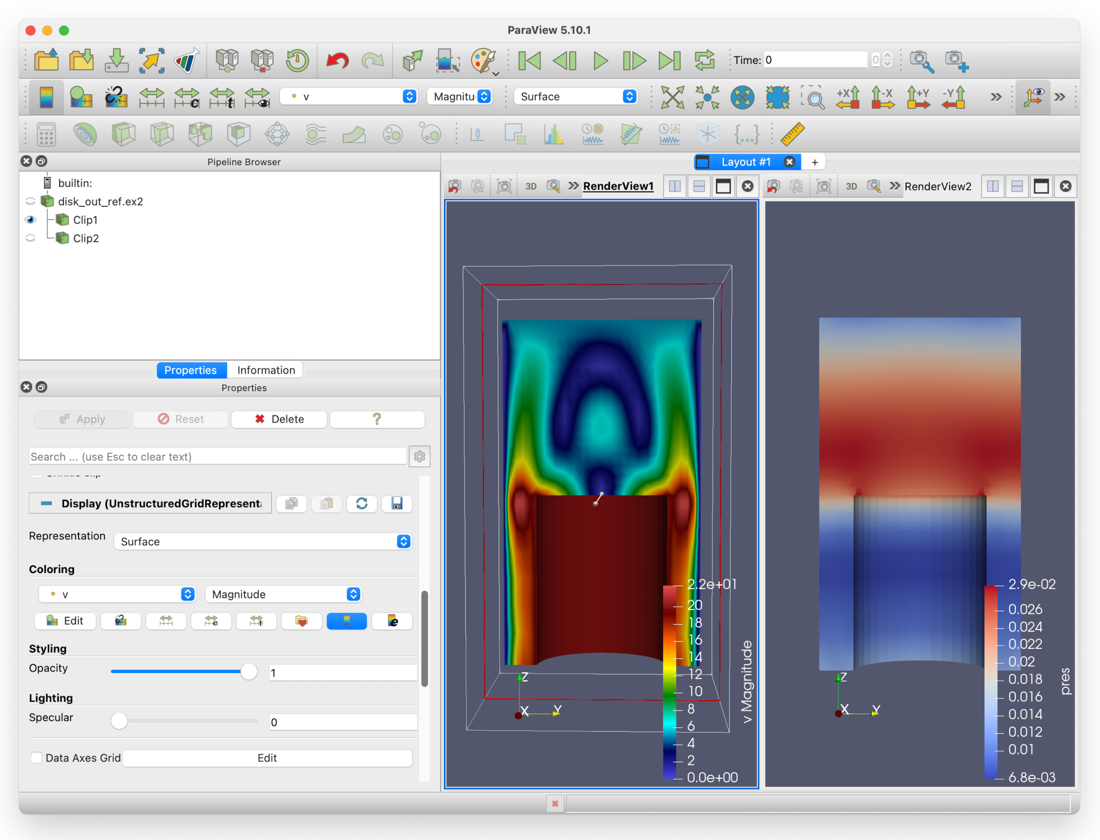
You should now see that the colourmap for the velocity magnitude in RenderView1 has changed.

Key Points

• Paraview can use filters to highlight specific aspects of the data

• Multiple filters can be used on one set of data

• Different views can be created to display different filters

• Colourmaps tell Paraview how to colour data fields

Saving your work

Overview

Teaching: 5 min
Exercises: 5 min

Questions

• How do I save my work?

Objectives

• Saving your progress

Saving your work

At this point, we have made a scene with a degree of complexity, that would take a considerable amount of time to recreate. Fortunately, Paraview has a way of preserving this for later - you could say, its saving grace - so that we can quit Paraview, do something else, and pick up where we left off later.

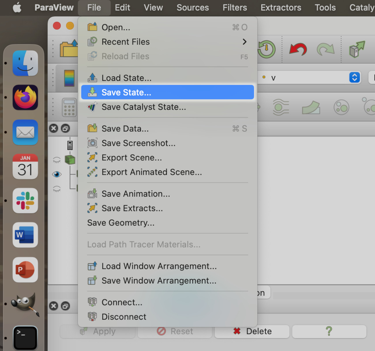
Paraview keeps a record of everything it has done in a session, so it records its State. We are going to use the Save State feature to save the state to disk.

You need to find the File menu and click on the Save State item. On Windows or Linux, this will be at the top of the application window, whereas on MacOS this will be at the top of the screen in the application menu:

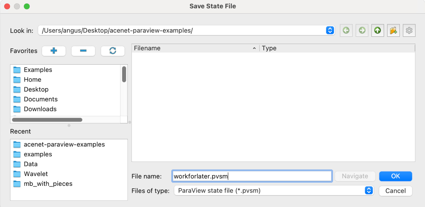
Paraview will show the save state dialogue. Here, the state file workforlater.pvsm will be saved to Desktop/acenet-paraview-examples/, but you can save the state file anywhere you like.

Unless you get an error message, your Paraview state should now be saved. If you’re feeling brave, you can now close Paraview.

(Suggested break: 15-20 minutes)

Key Points

• Paraview can save its entire state for later

Resuming a session

Overview

Teaching: 10 min
Exercises: 15 min

Questions

• How do I pick up where I left off?

Objectives

• Learning how to load a session

• Moving your session to another machine

Resuming a session

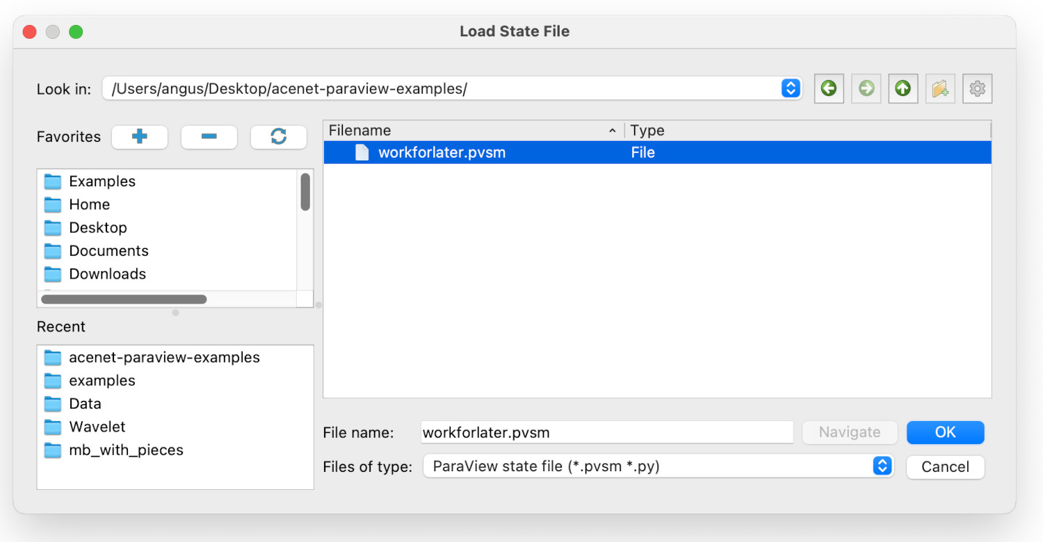
Assuming that you were brave/foolhardy enough to Save State and quit Paraview, we will now reload the saved session. After starting Paraview, find the Load State item in the File menu - it’s just above the Save State item. This will give you the load state dialogue window: navigate to where the state was saved, and select the state file you want to load, then clock Ok. In this case, the state file is at Desktop/acenet-paraview-examples/workforlater.pvsm.

This will give a second dialogue, named Load State Options. We will return to this later, but we can ignore it for now, as just click on Ok.

You should now have the original session, which you saved earlier.

You can continue using the session as you were before.

Potential problems

A state file is an precise record of what a Paraview session contained at the moment it was saved. That means that locations of external data sources, such as simulation results files, are saved too.

While this sounds convenient, if you are working on one system only, some concerns that could arise are:

• What happens if you want to use Paraview to look at your data on a different system?
• How do you do that, when the results files may be in a different place?

We will deal with those questions below.

Moving to Paraview on a different system

Let’s assume that you are now on a seperate computer, and you have copied across your data files, and your state file. We are going to start from scratch and load in your copied session on this new system.

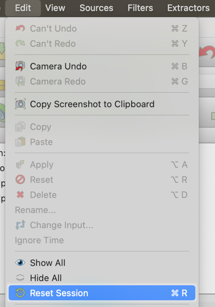
We will start from scratch. Go into the Edit menu and select the Reset Session item.

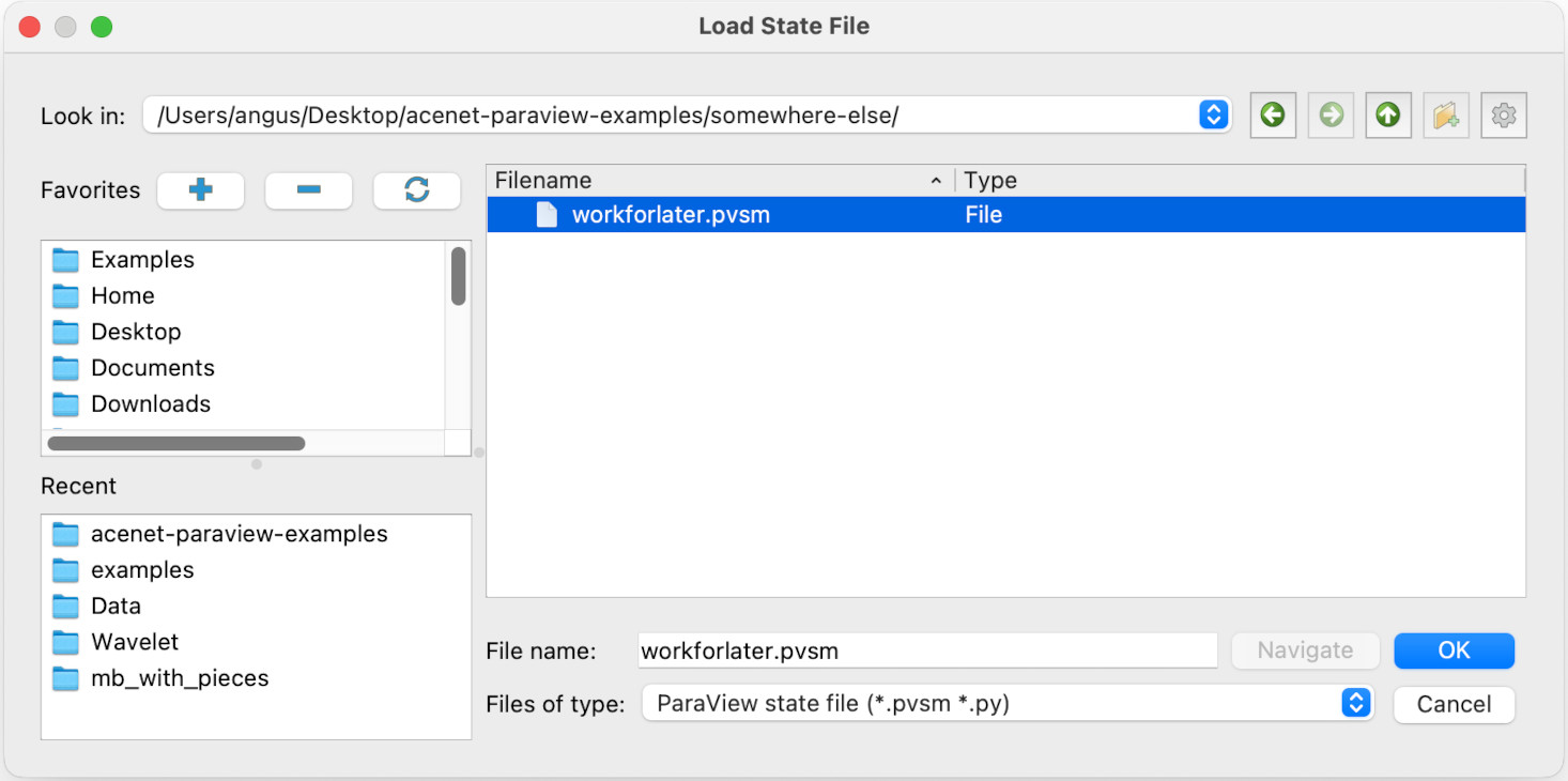
For this lesson, the state file and data file have been copied to Desktop/acenet-paraview-examples/somewhere-else/ to simulate the new computer we are opening our files on. We select the Load State item in the File menu, and select workforlater.pvsm, then click on Ok.

This takes you to the Load State Options dialogue. Here, we are going to change the option. In the pull-down menu, there are three options:

1. Use Files Names From State
2. Search files under specified directory
3. Choose File Names

We will pick Choose File Names. You will see the dialogue has changed to something like this:

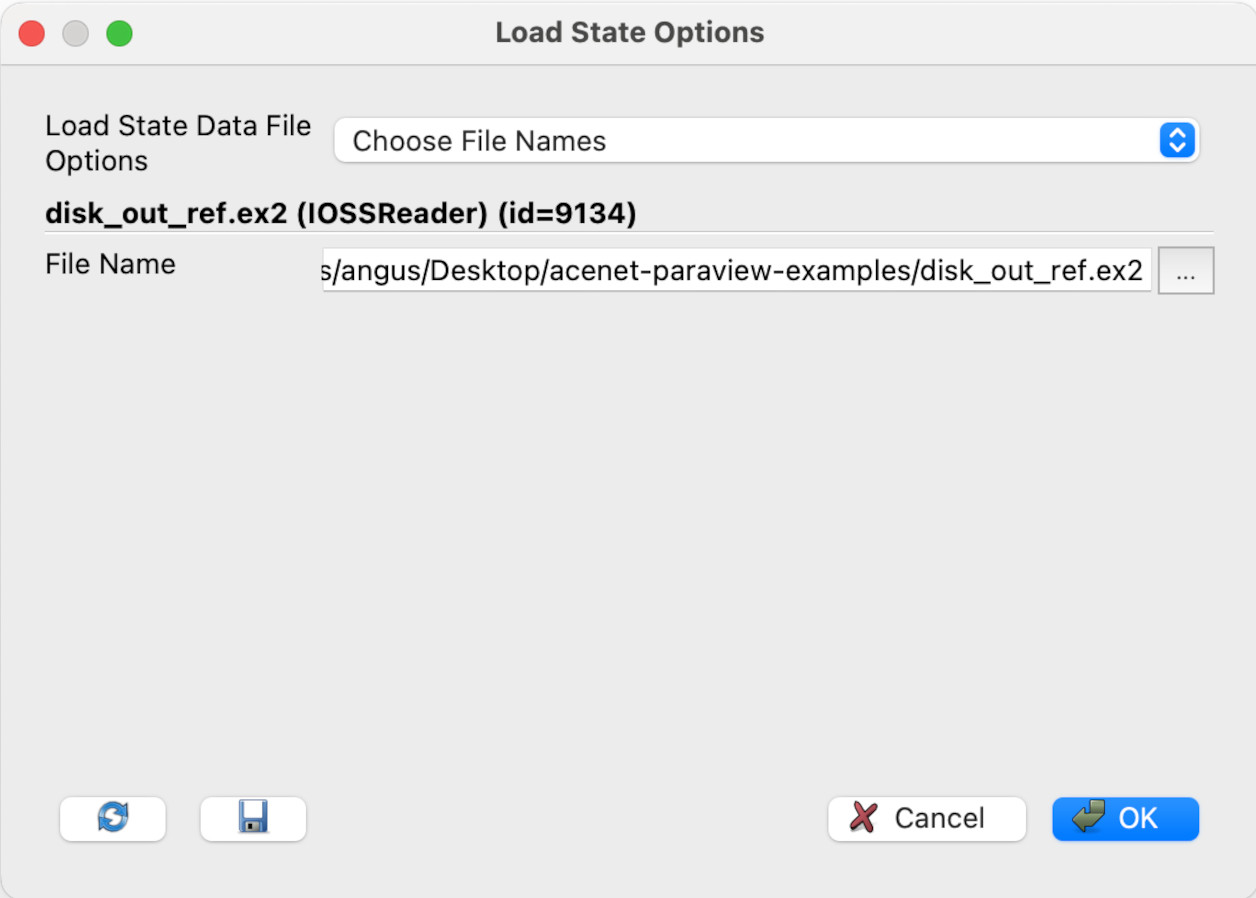
Click on the ellipsis (…). In the Select File Name dialogue, navigate to Desktop/acenet-paraview-examples/somewhere-else (or equivalent) and click on disk_out_ref.ex2, then click OK. Then click OK in the Load State Options dialogue.

(Alternately, you can just type the file name in the File Name text box if you know the file’s exact location.)

Your session should now be loaded with the new data file. As the location of the data file has changed, now would be a good time to save the session state to a new state file.

Key Points

• Session states can be loaded in.

• Take your sessions elsewhere, with caution

Introduction to working with real data

Overview

Teaching: 15 min
Exercises: 20 min

Questions

• How do I extract data from real data

Objectives

• Extracting data from multidimensional data

• Saving the data for external processing

Introduction

In this section, we will look at loading in data from an MRI scan of a human head.

Opening and viewing the file

• Click on File then Open.
• Navigation to the acenet-paraview-examples/ directory.
• Select the file mri-scan.pvd, then click OK.
• Click Apply in the Properties tab.

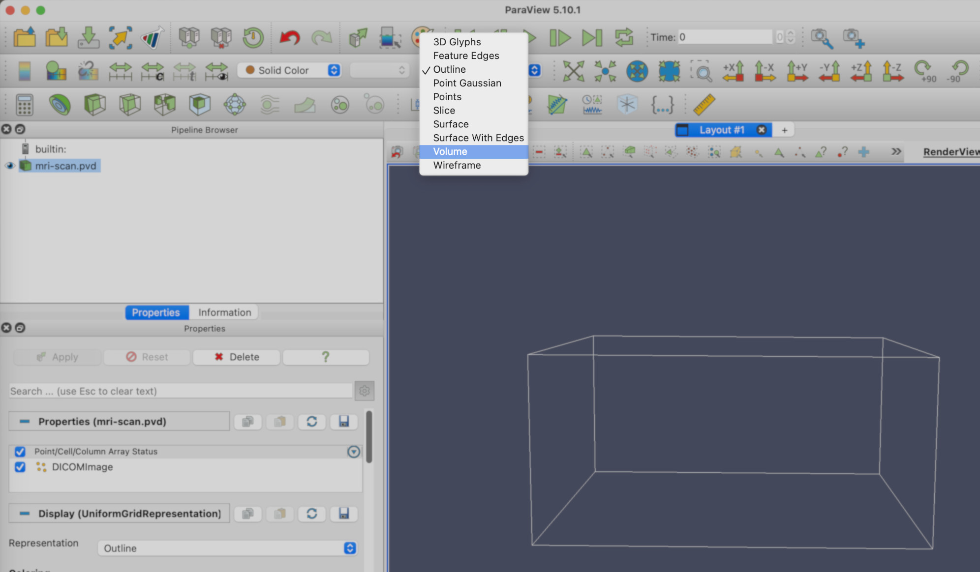
You should see a wireframe box. We’ll need to change the rendering to Volume. In the toolbar, you’ll see a drop-down menu that currently says Outline. Select Volume from this menu.

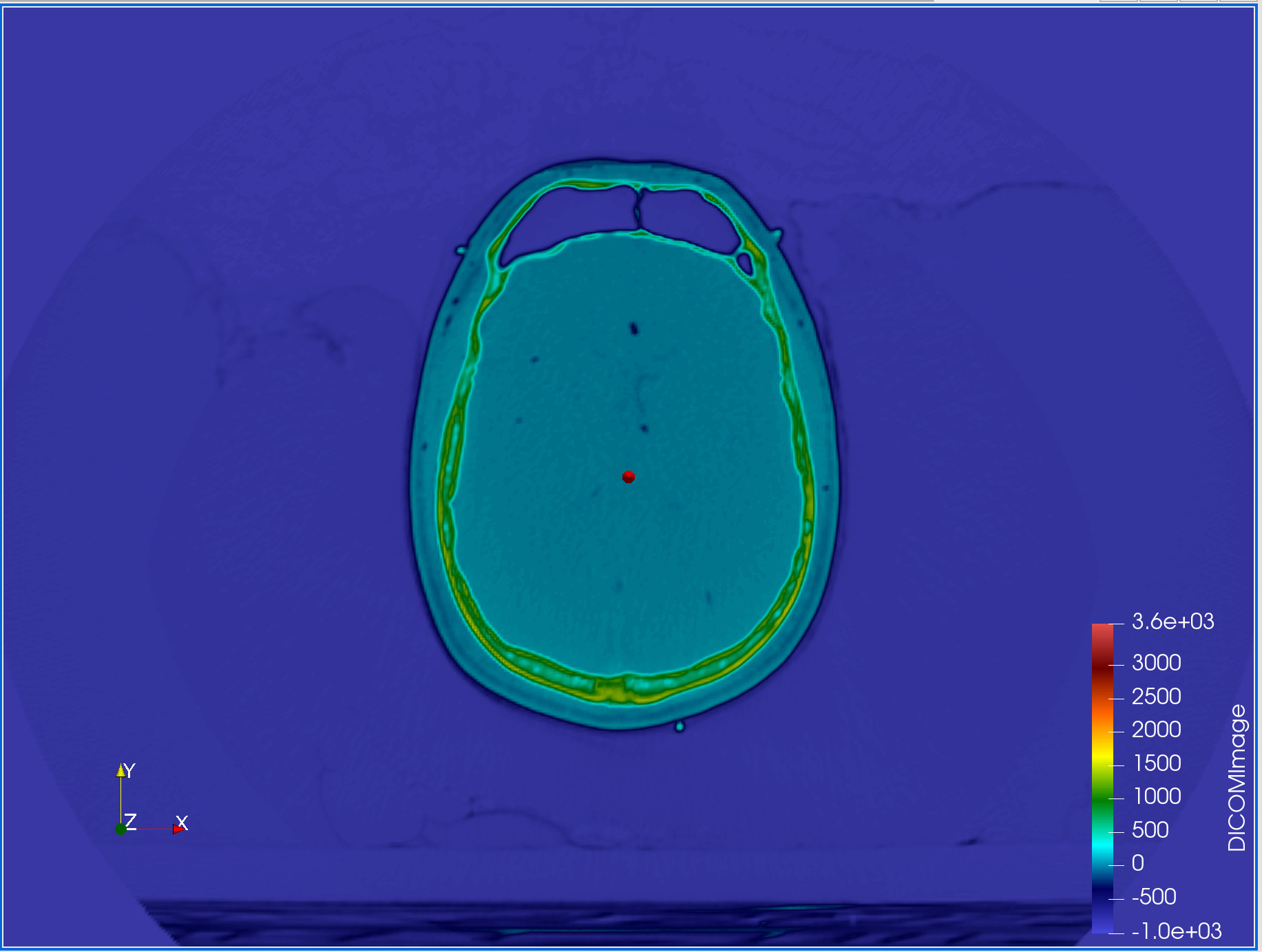
Zooming in a bit, you should have a view of the head clearly. Changing the colormap to Rainbow Desaturated (See the ‘Introducing filters’ episode, under Changing the colormap), and turning on the colormap legend, you should see something similar to this.

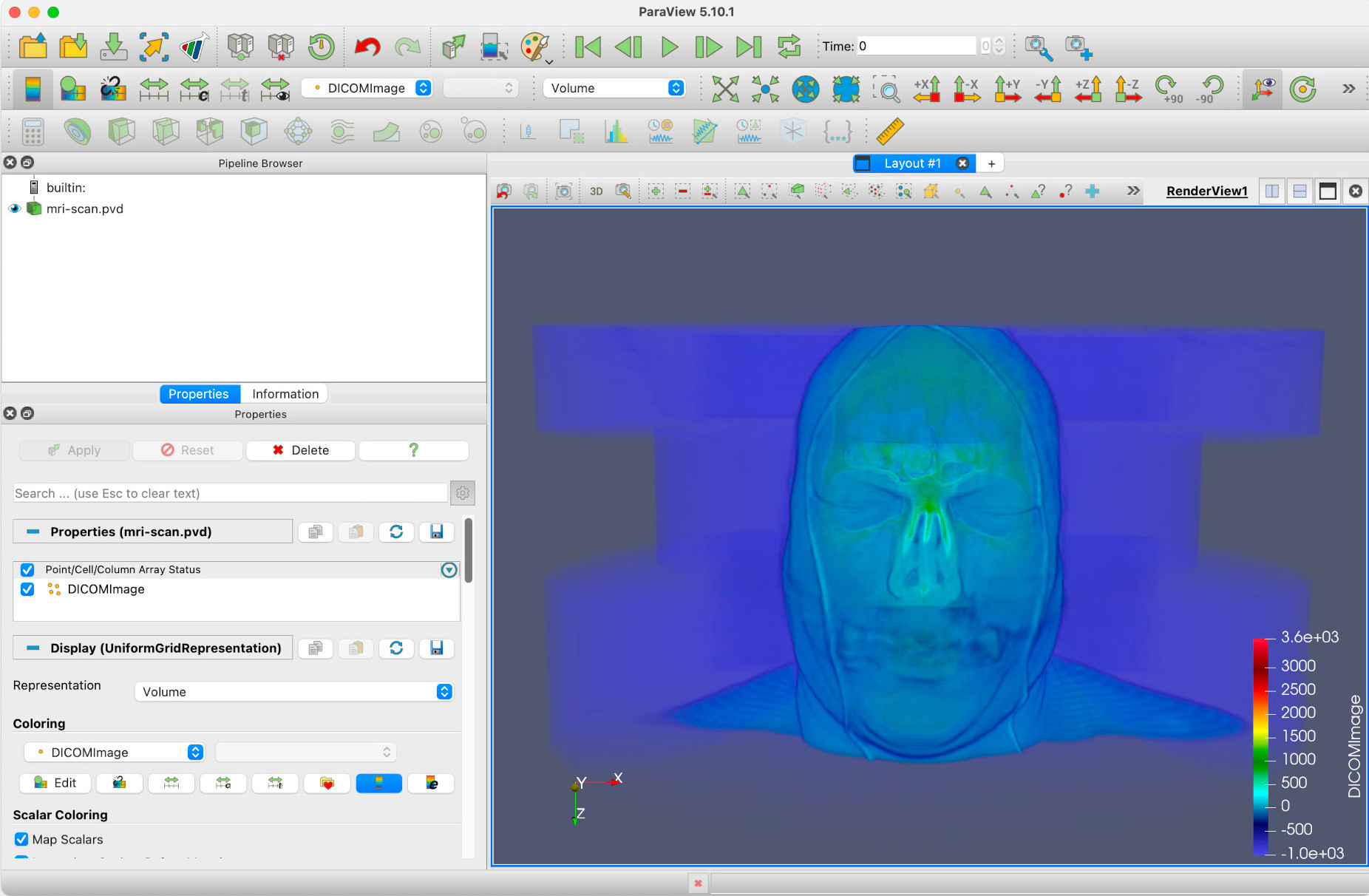
As the render type Volume suggests, this is a full volumetric render of 3D data. DICOM, incidentally, stands for Digital Imaging and Communications in Medicine, and is a standard for storing and transmitting medical images. More can be found on DICOM at the DICOM Library. For now though, we’ll treat the DICOMImage field in Paraview as a measure of object density.

Arranging and slicing the view

Paraview is not designed by default to deal with MRI scans, although it does support DICOM image sets. That said, we can still get useful information out of them. This we will do now.

Let’s suppose we want to get the horizontal dimensions of the head above the eyebrow. Firstly, we create a Slice filter, select Z Normal, then click Apply.

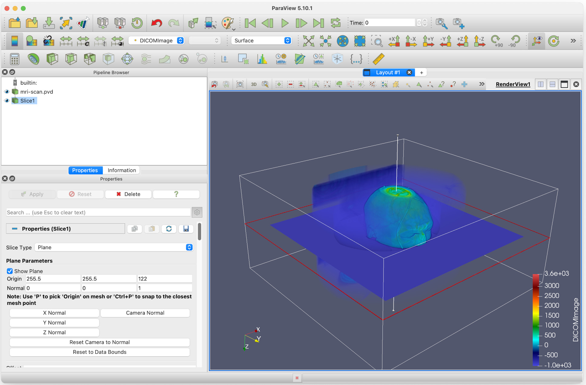
By clicking and dragging the red horizontal edge of the slice, we can move this to above the eyebrows of the head. Do this, and then:

• Uncheck Show Plane under Plane Parameters. This will stop the plane being moveable.
• Hide the original full 3D MRI image, by clicking on the eye icon next to mri-scan.pvd.
• Reorient the view to look down on the slice by clicking on the -Z axis icon in the toolbar.

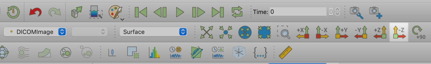
Zooming in a bit gives a clearer view in the main window.

Measuring

We are going to assume that green shell represents the skull, with the light blue being the outer layers of skin and tissue. We want to measure the cranium.

Firstly, we make the view 2D. We do this by click on the 3D button at the top of the main viewer window.

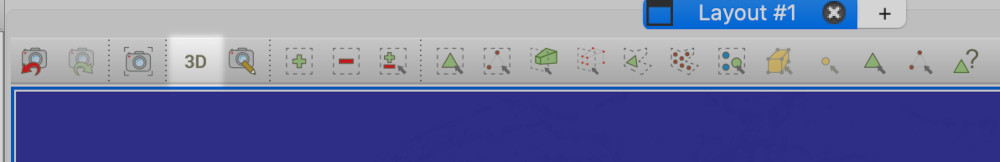
This will change the view to 2D, which makes our next tasks easier. You want to zoom in again at this point.

We want to measure the width of the cranium in the X direction. We can do this, and more, by adding a Plot Over Line filter.

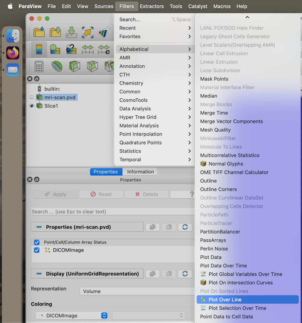
This will give us a matrix of values to enter the start and end points of the line.

• We want to make sure the line is visible on the screen, so it should be within the limits of the skull slice.
• In particular, the z-coordinates should be just above the slice.
• Click Apply.

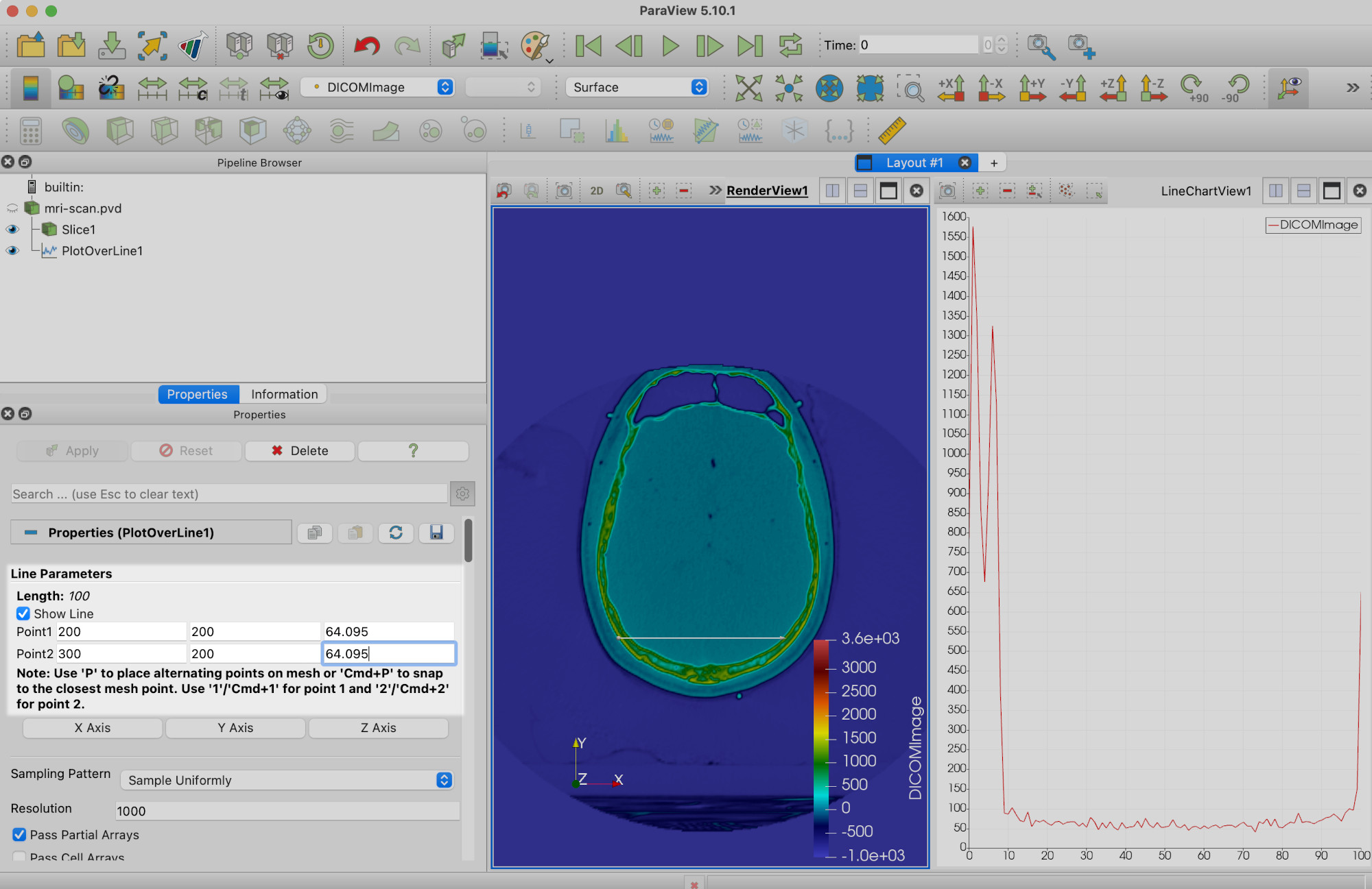
(You’ll note a line graph has appeared on the right hand side. We’ll get to this later.)

We’re now going to move the ends of the line to the widest part of the skull. You will need to click Apply once you have done so.

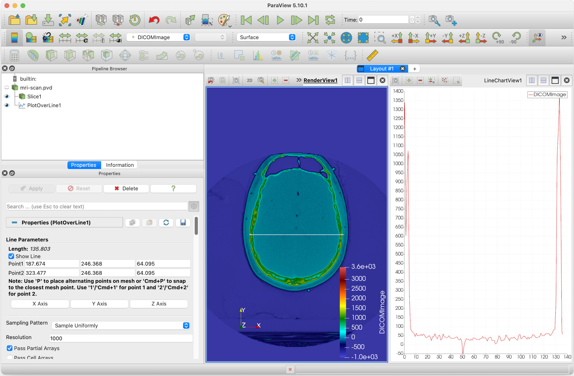
We can now see that under Line Parameters the width (here, length of line) is 135.803 units. But we can get more information than that.

Exporting the data

Returning our attention to the right hand view pane, LineChartView1, we can see that Paraview has plotted the values of DICOMImage along the length of the line.

This is data we can export for use elsewhere. First, we have to click on PlotOverLine1 within the Pipeline browser.

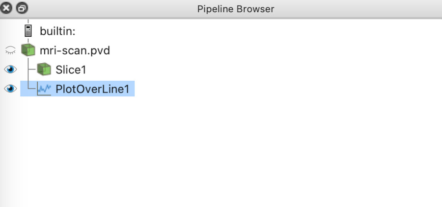
Then go into the File menu, and select Save Data. You’ll see this dialog window:

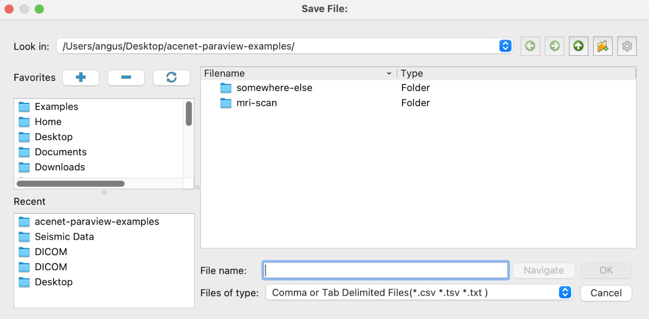
Notice that the file type is CSV. This is good: this is what we want. Once you have navigate to the directory you want to save in, enter your filename. We’ll call this one brain-sample.csv . Click on OK.

This will open another dialog. We don’t need anything but the defauts, so click OK again.

We now have a file we can use elsewhere. For instance, if you open it with Excel, you will see somethine like this -

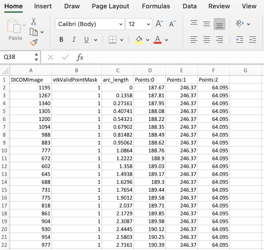
The column have been widened to see the column names. They are, in order:

• DICOMImage. This column contains the interpolated values of the field along the line. If there were multiple fields in the Paraview data, they would appear after this.
• vtkValidPointMask. A Paraview-specific diagnostic we don’t need to worry about it.
• arc_length . The length along the line of each point, moving from the beginning to end points.
• Points:0, :1, :2 . The x, y, and z co-ordinates of each point.

Summary

This is just a taste of what Paraview can do - more will be shown in the next section.

Key Points

• Paraview can work with other analysis tools by exporting data to file

• These files can be in a variety of formats used by other software (eg. CSV)

Working with large datasets on a cluster

Overview

Teaching: 15 min
Exercises: 0 min

Questions

• Running Paraview on HPC systems

Objectives

• Learn how Paraview works in client-server mode

Attention

This section will be a demonstration only.

You are not expected to recreate the tasks below during the lesson (unless you have a cluster handy). These have been tested on an ACENET cluster, and may need adaptation to work on other clusters. If you are technically-inclined, by all means do so; otherwise contact your system administrator.

Introduction

Here, we will see a demonstration of how Paraview can be run on an HPC system, using compute nodes to process the data, while being controlled from a desktop computer.

This involves running Paraview in what is called client-server mode.

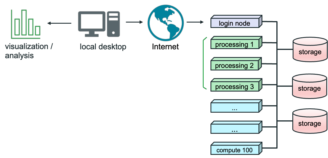
The diagram above shows how this works.

• The user on local desktop has the desktop version of Paraview.
• The server version of Paraview runs on the cluster, represented by the login and processing nodes on the right.
• The user connects to this through the Internet or local area network.
• Visualizations and data analysis are rendered on the user’s desktop.

Downloading and installing the Paraview on the cluster

The first task is to install headless mode Paraview on the HPC system you want to use. Headless mode means that this version of Paraview does not require a desktop, or even a graphics card. It is not designed for direct user interaction through a user interface; rather, it is designed as a server process which the user connects to with their own desktop Paraview.

On the Paraview download page, if you click on the Linux tab, you should see something similar to the following (may have to you scroll down slightly):

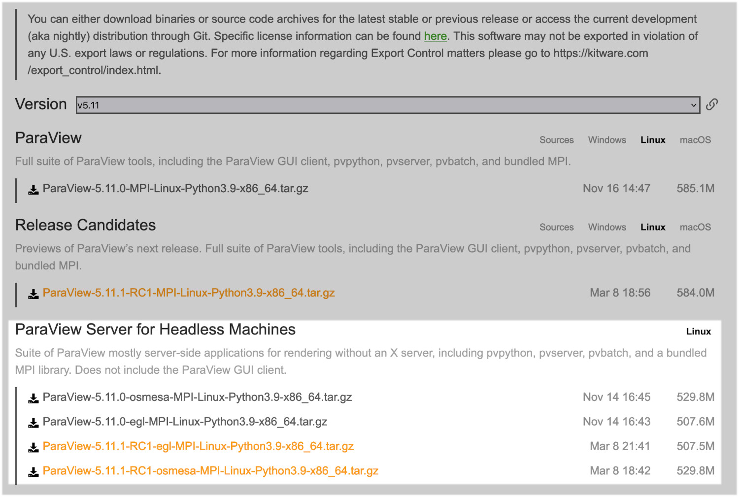
By default you should go for an osmesa version. This does not require a GPU to operate. If you have a cluster with GPUs, you can try an egl version. We will be using osmesa versions for this demonstration.

Once you have downloaded Paraview, extract the file archive where you can access it on the cluster. It can be installed under a user directory, as it does not need any special permssions.

Warning

The desktop and server version numbers of Paraview must be the same, otherwise Paraview will not work properly, if at all.

Running Paraview on the cluster

To run Paraview on an HPC cluster, you usually have to submit a batch job to the scheduler to run. This is what we will be doing here. Below is a simple Slurm batch script, which creates a job called ‘paraview’, which will run for 3 hours and uses 40 cores.

#!/bin/bash --login
#SBATCH --job-name=paraview
#SBATCH --time=3:0:0
#SBATCH --ntasks=40
#SBATCH --mem-per-cpu=2G
#SBATCH --output=para-%j.out
#SBATCH --error=para-%j.err

portnum=5002
paraver=5.10.1

echo "Starting Paraview headless servers on port $portnum"

paradir=$HOME/local/paraview/ParaView-5.10.1-osmesa-MPI-Linux-Python3.9-x86_64
parabin=$paradir/bin

export LD_LIBRARY_PATH=$paradir/lib/paraview-$paraver:$LD_LIBRARY_PATH
export PATH=$parabin:$PATH
export PYTHONPATH=$paradir/lib/paraview-$paraver/site-packages:$PYTHONPATH

srun $parabin/pvserver --force-offscreen-rendering --server-port=$portnum

echo "Paraview finished."

To adapt the Slurm script to your own cluster:

• In this case, we have installed Paraview under $HOME/local/paraview/ParaView-5.10.1-osmesa-MPI-Linux-Python3.9-x86_64. You may want to change paradir if you install to another directory.
• Change paraver to match the version you use.
• If 40 cores are insufficient, you may need to change ntasks to something larger.
• If you are not using Slurm as a scheduler, you will need to change the formatting, and the Slurm batch directives (#SBATCH).
• If your cluster has nodes with M cores each, make sure ntasks is a multiple of M.

We will be running on 40 cores, which is sufficient for many data sets. The Paraview server will be running on port number 5002.

Once that script is written to file (we will call it viz.slurm), then it is submitted to the scheduler with the command

sbatch viz.slurm

This will give the message Submitted batch job XXXX where XXXX is the job number. If we then run

squeue -u $USER

Then we can see if it is running. A message similar to this should appear:

          JOBID     USER      ACCOUNT           NAME  ST  TIME_LEFT NODES CPUS TRES_PER_N MIN_MEM NODELIST (REASON) 
         431486  my_user        staff       paraview   R    2:59:58     1   40        N/A      2G cl005 (None) 

This tells us that Paraview is running (the ‘R’ under State, or ST), and that I am using 1 node. The node here is given as cl005. This should be noted down, as it will be required in a moment.

Connecting to Paraview on the cluster

Before we can run Paraview on our desktop, we need to connect to the cluster with SSH, and with a SSH tunnel in place. The techniques here will work under Linux and MacOS, but need modification for use under Windows (eg. if using Putty).

What we are going to do is open a local port on our desktop, that connect directly to the compute node on the cluster where the Paraview server processes are running.

We do this (from our MacOS or Linux desktop) by issuing the following command at the terminal prompt

ssh my_user@cluster.address.ca -L 5002:cl060:5002

This opens port 5002 on our desktop, and pipes it to port 5002 on cl060 on the cluster. You will need to change this name to whatever node the scheduler has allocated your Paraview job to.

Now we can fire up Paraview on our desktop. If you select Connect under the File menu, you should see this dialog:

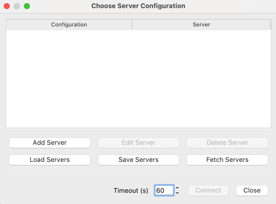
We want to click on Add Server. This will give the Edit Server Configuration dialog.

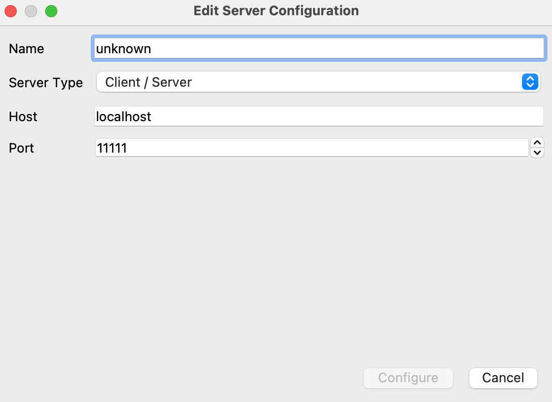
Change the name to something convenient, and the port to 5002, then click Configure. This gives a further dialog on launch options - just click Save. Now we can choose a server to connect to:

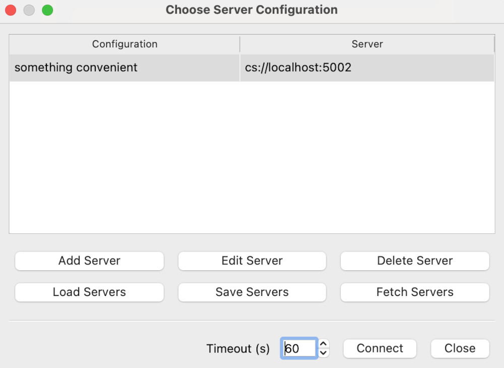
Here, we want to select the server connection we’ve just created, and hit Connect. This may take a few moments.

Once connected, you can open files within Paraview, apply filters and even export data exactly as if you were using Paraview only on your desktop.

Instructor demonstration

The instructor will conduct a short demonstration on using Paraview on a cluster. This will be using datasets much larger than can be conveniently processed on a desktop.

Key Points

• Running Paraview in client/server mode allows remote visualization of large data sets.

• The Paraview client connects to the Paraview server processes on the cluster.

• The size of these datasets is only limited by server-side resources.

Concluding remarks

Overview

Teaching: 10 min
Exercises: 0 min

Questions

• What now?

Objectives

• Learn where to find more information.

Going beyond the basics

Hopefully this tutorial has given you a taste of what Paraview is capable of. Paraview can do much more than demonstrated here, and applied in many more areas or disciplines than detailed in this tutorial.

One aspect that is worthy of further exploration is that of Paraview’s Python interface. This allows the user to embed Python within Paraview, so that they can draw in their own analysis tools and integrate them with Paraview. This is very powerful, as it allows effectively allows Paraview’s functionality to be extended far beyond its already sizeable tool set.

Furthermore, Paraview can be run without the graphical user interface at all, and process data in batch mode. To do this, the command pvpython is used. This is a particularly useful option for processing large datasets on HPC clusters.

If you are interested in exploring Paraview further, one of the best places to start is the official Paraview User Guide. This can be found at:

• docs.paraview.org/en/latest/UsersGuide

In addition there are the self-directed tutorials, which will walk you through all aspects of Paraview. You can find those here:

• docs.paraview.org/en/latest/Tutorials/SelfDirectedTutorial

Wishing you the best in your future Paraview endeavours,

– The ACENET team.

Key Points

• Paraview is well documented.

• The ParaView Users’s Guide has extensive information.