Thinking in Parallel

Overview

Teaching: 30 min
Exercises: 15 min

Questions

• How do I re-think my algorithm in parallel?

Objectives

• Take the MD algorithm from the profiling example and think about how this could be implemented in parallel.

Our Goals

• Don’t duplicate work.
• Run as much as possible in parallel.
• Keep all CPU-cores busy at all times.
• Avoid processes/threads having to wait long for data.

What does that mean in terms of our MD algorithm?

Sequential Algorithm

The key subroutine in the sequential MD code, we discovered in the previous episode, is compute(...). You can find it at line 225 of md_gprof.f90, and the major loop begins at line 295. Written in Python-ish pseudo-code the whole program looks something like this:

Pseudo Code

initialize()
step = 0

while step < numSteps:

  for ( i = 1;  i <= nParticles; i++ ):
    for ( j = 1;  j <= nParticles; j++ ):
      if ( i != j ) :
        calculate_distance(i, j)
        calculate_potential_energy(i, j)
        # Attribute half of the total potential energy of this pair to particle J.

        calculate_force(i, j)
        # Add particle J's contribution to the force on particle I.

  calculate_kinetic_energy()
  update_velocities()
  update_coordinates()

finalize()

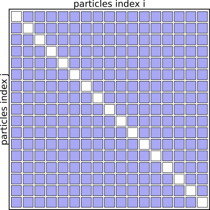
The algorithm basically works through a full matrix of size $N_{particles}^2$, evaluating the distances, potential energies and forces for all pairs (i,j) except for (i==j).

Graphically it looks like this:

Interaction Matrix: pair interactions (i!=j)

Step 1: Improve the sequential code

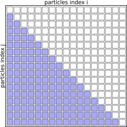
If you understand the problem domain well enough— and maybe you do, if the pseudo-code makes sense to you already— then you might notice that that interaction matrix will always be symmetrical. We don’t need to evaluate the pairs of particles twice for (i,j) and (j,i), as the contribution to the potential energy for both is always the same, as is the magnitude of the force for this interaction, just the direction will always point towards the other particle.

We can basically speed up the algorithm by a factor of 2 just by eliminating redundant pairs and only evaluating pairs (i<j)

Pseudo Code

initialize()
step = 0

while step < numSteps:

  for ( i = 1;  i <= nParticles; i++ ):
    for ( j = 1;  j <= nParticles; j++ ):
      if ( i < j ):
        calculate_distance(i, j)
        calculate_potential_energy(i, j)
        # Attribute the full potential energy of this pair to particle J.

        calculate_force(i, j)
        # Add the force of pair (I,J) to both particles.

  calculate_kinetic_energy()
  update_velocities()
  update_coordinates()

finalize()

Interaction Matrix: pair interactions (i<j)

Another way to express the same idea is not to check for i<j at each iteration, but to recode the inner loop to only start counting from i+1, like this:

Pseudo Code

...
  for ( i = 1;  i <= nParticles; i++ ):
    for ( j = i + 1;  j <= nParticles; j++ ):
...

At this point, properly we should modify the code, re-compile the program, and profile it again to find out if our “hot spots” have changed. We’re not going to take time to do that today. Take my word for it that the compute function is still the costliest, and that calc_distance and calc_force are still the major contributors inside of compute.

Step 2: Parallelize the outer loop

It’s not 100% reliable, but a good rule when parallelizing code is to start with the outermost loop in your “hot spot”. Following that rule in this example, a good thing to try would be to turn the outer for-loop (over index i) into a parallel loop. The work for columns i=1,2 will be assigned to core 1, columns i=3,4 to core 2, and so on. (We will show you how to actually implement this e.g. using OpenMP in later days of the workshop.)

Pseudo Code

initialize()
step = 0

while step < numSteps:

  # Run this loop in parallel:
  for ( i = 1;  i <= nParticles; i++ ):
    for ( j = i + 1;  j <= nParticles; j++ ):
        calculate_distance(i, j)
        calculate_potential_energy(i, j)
        # Attribute the full potential energy of this pair to particle J.

        calculate_force(i, j)
        # Add the force if pair (I,J) to both particles.
  gather_forces_and_potential_energies()

  # Continue sequentially:
  calculate_kinetic_energy()
  update_velocities()
  update_coordinates()
  communicate_new_coordinates_and_velocities()

finalize()

We need to add a step, gather_forces_and_potential_energies because eventually every particle has to know about every other particle, no matter which processor the particle is assigned to. That’s not a problem.

Question

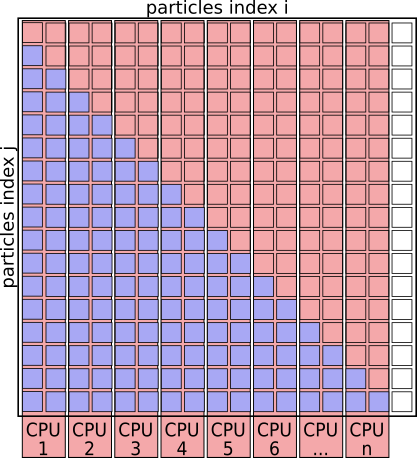
There is a different and subtle problem with this scheme. Can you see it in this picture of the interaction matrix?

Interaction Matrix: with simple parallelization

Answer

With this scheme core 1 will be responsible for many more interactions than core 8. So our CPU cores are, on average, idle about 50% of the time, and the whole solution is not available until the most-loaded process finishes.

This can be improved by creating a list of particle pairs, and then distribute that list of particle-pairs evenly between cores for evaluation.

Pseudo Code: Using pair-list

initialize()
step = 0

while step < numSteps:

  # generate pair-list
  pair_list = []
  for ( i = 1;  i <= nParticles; i++ ):
    for ( j = i+1;  j <= nParticles; j++ ):
      pair_list.append( (i,j) )

  # Run this loop in parallel:
  for (i, j) in pair_list:
    calculate_distance(i, j)
    calculate_potential_energy(i, j)
    # Attributing the full potential energy of this pair to particle J.

    calculate_force(i, j)
    # Add the force if pair (I,J) to both particles.
  gather_forces_and_potential_energies()

  # Continue sequentially:
  calculate_kinetic_energy()
  update_velocities()
  update_coordinates()
  communicate_new_coordinates_and_velocities()

finalize()

Using cut-offs

We expect this algorithm to scale as $N_{particles}^2$; that is, the amount of work to be done goes up as the square of the number of particles. The things we’ve done so far haven’t changed that, although we have reduced the amount of work one needs to do per particle pair.

Can we do better? Is there a way to make the amount of work grow more slowly than $N_{particles}^2$?

Once again, knowledge of the problem domain and the algorithm is essential.

At large distances the force between two particles becomes extremely small, and the contribution of the pair to the potential energy likewise becomes small. There must be some distance beyond which all forces and potential-energy contributions are “effectively” zero. Recall that calc_pot and calc_force were expensive functions in the profile we made of the code earlier, so we can save time by not calculating these if the distance we compute is larger than some suitably-chosen $r_{cutoff}$.

Further optimizations can be made by avoiding to compute the distances for all pairs at every step - essentially by keeping neighbor lists and using the fact that particles travel only small distances during a certain number of steps. However, those are beyond the scope of this lesson and are well described in text-books, journal publications and technical manuals.

Spatial- (or Domain-) Decomposition

The scheme we’ve just described, where each particle is assigned to a fixed processor, is called the Force-Decomposition or Particle-Decomposition scheme. When simulating large numbers of particles (~ 10⁵) and using many processors, communicating the updated coordinates, forces, etc., every timestep can become a bottle-neck with this scheme.

To reduce the amount of communication between processors we can partition the simulation box along its axes into smaller domains. The particles are then assigned to processors depending on in which domain they are currently located. This way many pair-interactions will be local within the same domain and therefore handled by the same processor. For pairs of particles that are not located in the same domain, we can use e.g. the “eighth shell” method in which a processor handles those pairs in which the second particle is located only in the positive direction of the dimensions, as illustrated below.

Domain Decomposition using Eight-Shell method

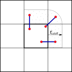
In this way, each domain only needs to communicate with neighboring domains in one direction— as long as the shortest dimension of a domain is larger than the longest cut-off distance.

Domain Decomposition not only applies to Molecular Dynamics (MD) but also to Computational Fluid Dynamics (CFD), Finite Elements methods, Climate- & Weather simulations and many more.

MD Literature:

1. Larsson P, Hess B, Lindahl E.; Algorithm improvements for molecular dynamics simulations.
   Wiley Interdisciplinary Reviews: Computational Molecular Science 2011; 1: 93–108. doi:10.1002/wcms.3
2. Allen MP, Tildesley DJ; Computer Simulation of Liquids. Second Edition. Oxford University Press; 2017.
3. Frenkel D, Smit B; Understanding Molecular Simulation: From Algorithms to Applications. 2nd Edition. Academic Press; 2001.

Load Distribution

Generally speaking, the goal is to distribute the work across the available resources (processors) as evenly as possible, as this will result in the shortest amount of time and avoids some resources being left unused.

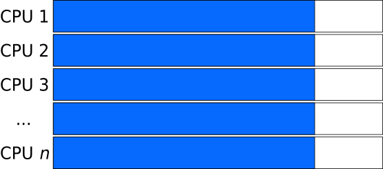
Ideal Load: all tasks have the same size

An ideal load distribution might look like this:

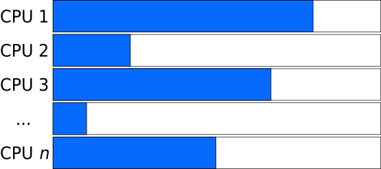
Unbalanced Load: Tasks of different sizes

Whereas if the tasks that are distributed have varying length, the program needs to wait for the slowest task to finish.

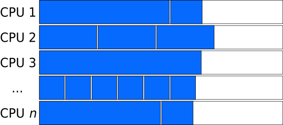
Balanced Load: Combining long and short tasks

If you have many more independent tasks than processors, and if you can estimate the lengths of the tasks easily, then you may be able to combine tasks of different lengths into “chunks” of similar length to balance the load:

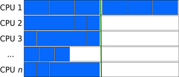
Number of chunks a multiple of number of processors

Chunks consisting of many tasks can result in consistent lengths of the chunks, if you are careful (or lucky).

But larger chunks implies a smaller number of chunks. This can cause another inefficiency if the number of chunks is not an integer multiple of the number of processors. In the figure below, for example, the number of chunks is just one larger than the number of processors, so $N-1$ processors are left idle while the $N+1$th chunk is finished up.

Task-queues

Creating a queue (list) of independent tasks which are processed asynchronously can improve the utilization of resources, especially if the tasks can be sorted from longest to shortest.

However, care needs to be taken to avoid a race condition in which two processes take the same task from the task-queue. Having a dedicated manager process to assign the work to the compute processes can eliminate the race-condition, but introduces more overhead (mostly the extra communication required) and can potentially become a bottle-neck when a very large number of processes are involved.

Generally speaking there is a trade-off: Smaller chunks lead to better load balancing, and are hence more efficient. But smaller chunks also usually require more communication (or total storage, or other forms of parallel overhead), and so are less efficient. Assuming you have any choices about chunk size at all, the “best” chunk size for your problem can probably only be determined by trying things.

Key Points

• Adapting a sequential code so it will run efficiently parallel needs both planning and experimentation.

• It is vital to first understand both the problem and the sequential algorithm.

• Shorter independent tasks need more overall communication.

• Longer tasks and large variations in task-length can cause resources to be left unused.

• Domain Decomposition can be used in many cases to reduce communication by processing short-range interactions locally.

• There are many textbooks and publications that describe different parallel algorithms. Try finding existing solutions for similar problems.