Analyzing Performance Using a Profiler
Overview
Teaching: 30 min
Exercises: 20 minQuestions
How do I decide where to begin optimizing my code?
Objectives
Use a profiler to analyze the runtime behaviour of a program.
Identify areas of the code with potential for optimization and/or parallelization.
Programmers often tend to over-think design and might spend a lot of their time optimizing parts of the code that only contributes a small amount to the total runtime. It is easy to misjudge the runtime behaviour of a program.
What parts of the code to optimize?
To make an informed decision what parts of the code to optimize, one can use a performance analysis tool, or short “profiler”, to analyze the runtime behaviour of a program and measure how much CPU-time is used by each function.
We will analyze an example program, for simple Molecular Dynamics (MD) simulations, with the GNU profiler Gprof. There are different profilers for many different languages available and some of them can display the results graphically. Many Integrated Development Environments (IDEs) also include a profiler. A wide selection of profilers is listed on Wikipedia.
Molecular Dynamics Simulation
The example program performs simple Molecular Dynamics (MD) simulations of particles interacting with a simple harmonic potential of the form:
\[v(x) = ( sin ( min ( x, \pi/2 ) ) )^2\]It is a modified version of an MD example written in Fortran 90 by John Burkardt and released under the GNU LGPL license.
Every time step, the MD algorithm essentially calculates the distance, potential energy and force for each pair of particles as well as the kinetic energy for the system. Then it updates the velocities based on the acting forces and updates the coordinates of the particles based on their velocities.
Functions in md_gprof.f90
The MD code md_gprof.f90 has been modified from John Burkardt’s version
by splitting out the computation of the distance, force, potential- and
kinetic energies into separate functions, to make for a more interesting
and instructive example to analyze with a profiler.
| Name of Subroutine | Description |
|---|---|
| MAIN | is the main program for MD. |
| INITIALIZE | initializes the positions, velocities, and accelerations. |
| COMPUTE | computes the forces and energies. |
| CALC_DISTANCE | computes the distance of a pair of particles. |
| CALC_POT | computes the potential energy for a pair of particles. |
| CALC_FORCE | computes the force for a pair of particles. |
| CALC_KIN | computes the kinetic energy for the system. |
| UPDATE | updates positions, velocities and accelerations. |
| R8MAT_UNIFORM_AB | returns a scaled pseudo-random R8MAT. |
| S_TO_I4 | reads an integer value from a string. |
| S_TO_R8 | reads an R8 value from a string. |
| TIMESTAMP | prints the current YMDHMS date as a time stamp. |
Regular invocation:
For the demonstration we are using the example md_gprof.f90.
# Download the source code file:
$ wget https://acenet-arc.github.io/ACENET_Summer_School_General/code/profiling/md_gprof.f90

# Compile with gfortran:
$ gfortran md_gprof.f90  -o md_gprof

# Run program with the following parameters:
#  2 dimensions, 200 particles, 500 steps, time-step: 0.1
$ ./md_gprof 2 200 500 0.1
25 May 2018   4:45:23.786 PM

MD
  FORTRAN90 version
  A molecular dynamics program.

  ND, the spatial dimension, is        2
  NP, the number of particles in the simulation is      200
  STEP_NUM, the number of time steps, is      500
  DT, the size of each time step, is   0.100000

  At each step, we report the potential and kinetic energies.
  The sum of these energies should be constant.
  As an accuracy check, we also print the relative error
  in the total energy.

      Step      Potential       Kinetic        (P+K-E0)/E0
                Energy P        Energy K       Relative Energy Error

         0     19461.9         0.00000         0.00000
        50     19823.8         1010.33        0.705112E-01
       100     19881.0         1013.88        0.736325E-01
       150     19895.1         1012.81        0.743022E-01
       200     19899.6         1011.14        0.744472E-01
       250     19899.0         1013.06        0.745112E-01
       300     19899.1         1015.26        0.746298E-01
       350     19900.0         1014.37        0.746316E-01
       400     19900.0         1014.86        0.746569E-01
       450     19900.0         1014.86        0.746569E-01
       500     19900.0         1014.86        0.746569E-01

  Elapsed cpu time for main computation:
     19.3320     seconds

MD:
  Normal end of execution.

25 May 2018   4:45:43.119 PM
Compiling with profiling enabled
To enable profiling with the compilers of the GNU Compiler Collection, we
just need to add the -pg option to the gfortran, gcc or g++ command.
When running the resulting executable, the profiling data will be stored
in the file gmon.out. Invoking gprof will then give us a profile.
By default, gprof looks for a data file named gmon.out but needs to
be given the name of the executable as an argument.
We can also use a larger number of particles and more time steps if we want a longer run time.
# Compile with GFortran with -pg option:
$ gfortran md_gprof.f90 -o md_gprof -pg

$ ./md_gprof 2 500 1000 0.1
# ... skipping over output ...

$ /bin/ls -F
gmon.out  md_gprof*  md_gprof.f90
# Now the file gmon.out has been created.

# Run gprof to view the output:
$ gprof ./md_gprof | less
Gprof then displays the profiling information in two tables along with an extensive explanation of their content. We will analyze the tables in the following subsections:
Flat Profile:
Flat profile:

Each sample counts as 0.01 seconds.
  %   cumulative   self              self     total
 time   seconds   seconds    calls   s/call   s/call  name
 39.82      1.19     1.19 19939800     0.00     0.00  calc_force_
 37.48      2.31     1.12 19939800     0.00     0.00  calc_pot_
 17.07      2.82     0.51 19939800     0.00     0.00  calc_distance_
  4.68      2.96     0.14      501     0.00     0.01  compute_
  1.00      2.99     0.03      501     0.00     0.00  calc_kin_
  0.00      2.99     0.00      500     0.00     0.00  update_
  0.00      2.99     0.00        3     0.00     0.00  s_to_i4_
  0.00      2.99     0.00        2     0.00     0.00  timestamp_
  0.00      2.99     0.00        1     0.00     2.99  MAIN__
  0.00      2.99     0.00        1     0.00     0.00  initialize_
  0.00      2.99     0.00        1     0.00     0.00  r8mat_uniform_ab_
  0.00      2.99     0.00        1     0.00     0.00  s_to_r8_
| Column | Description |
|---|---|
| % time | the percentage of the total running time of the program used by this function. |
| cumulative seconds | a running sum of the number of seconds accounted for by this function and those listed above it. |
| self seconds | the number of seconds accounted for by this function alone. This is the major sort for this listing. |
| calls | the number of times this function was invoked, if this function is profiled, else blank. |
| self s/call | the average number of milliseconds spent in this function per call, if this function is profiled, else blank. |
| total s/call | the average number of milliseconds spent in this function and its descendents per call, if this function is profiled, else blank. |
| name | the name of the function. This is the minor sort for this listing. |
In this example, the most time is spent computing the forces and potential energy. Calculating the distance between the particles is at 3rd rank and roughly 2x faster than either of the above.
Call Graph:
The Call Graph table describes the call tree of the program, and was sorted by the total amount of time spent in each function and its children.
			Call graph


granularity: each sample hit covers 2 byte(s) for 0.33% of 2.99 seconds

index % time    self  children    called     name
                0.14    2.85     501/501         MAIN__ [2]
[1]    100.0    0.14    2.85     501         compute_ [1]
                1.19    0.00 19939800/19939800     calc_force_ [4]
                1.12    0.00 19939800/19939800     calc_pot_ [5]
                0.51    0.00 19939800/19939800     calc_distance_ [6]
                0.03    0.00     501/501         calc_kin_ [7]
-----------------------------------------------
                0.00    2.99       1/1           main [3]
[2]    100.0    0.00    2.99       1         MAIN__ [2]
                0.14    2.85     501/501         compute_ [1]
                0.00    0.00     500/500         update_ [8]
                0.00    0.00       3/3           s_to_i4_ [9]
                0.00    0.00       2/2           timestamp_ [10]
                0.00    0.00       1/1           s_to_r8_ [13]
                0.00    0.00       1/1           initialize_ [11]
-----------------------------------------------
                                                 <spontaneous>
[3]    100.0    0.00    2.99                 main [3]
                0.00    2.99       1/1           MAIN__ [2]
-----------------------------------------------
                1.19    0.00 19939800/19939800     compute_ [1]
[4]     39.8    1.19    0.00 19939800         calc_force_ [4]
-----------------------------------------------
                1.12    0.00 19939800/19939800     compute_ [1]
[5]     37.5    1.12    0.00 19939800         calc_pot_ [5]
-----------------------------------------------
                0.51    0.00 19939800/19939800     compute_ [1]
[6]     17.1    0.51    0.00 19939800         calc_distance_ [6]
-----------------------------------------------
                0.03    0.00     501/501         compute_ [1]
[7]      1.0    0.03    0.00     501         calc_kin_ [7]
-----------------------------------------------
                0.00    0.00     500/500         MAIN__ [2]
[8]      0.0    0.00    0.00     500         update_ [8]
-----------------------------------------------
                0.00    0.00       3/3           MAIN__ [2]
[9]      0.0    0.00    0.00       3         s_to_i4_ [9]
-----------------------------------------------
                0.00    0.00       2/2           MAIN__ [2]
[10]     0.0    0.00    0.00       2         timestamp_ [10]
-----------------------------------------------
                0.00    0.00       1/1           MAIN__ [2]
[11]     0.0    0.00    0.00       1         initialize_ [11]
                0.00    0.00       1/1           r8mat_uniform_ab_ [12]
-----------------------------------------------
                0.00    0.00       1/1           initialize_ [11]
[12]     0.0    0.00    0.00       1         r8mat_uniform_ab_ [12]
-----------------------------------------------
                0.00    0.00       1/1           MAIN__ [2]
[13]     0.0    0.00    0.00       1         s_to_r8_ [13]
-----------------------------------------------
Each entry in this table consists of several lines. The line with the index number at the left-hand margin lists the current function. The lines above it list the functions that called this function, and the lines below it list the functions this one called.
This line lists:
| Column | Description |
|---|---|
| index | A unique number given to each element of the table. |
| % time | This is the percentage of the `total’ time that was spent in this function and its children. |
| self | This is the total amount of time spent in this function. |
| children | This is the total amount of time propagated into this function by its children. |
| called | This is the number of times the function was called. |
| name | The name of the current function. The index number is printed after it. |
Index by function name:
Index by the function name

   [2] MAIN__                  [5] calc_pot_               [9] s_to_i4_
   [6] calc_distance_          [1] compute_               [13] s_to_r8_
   [4] calc_force_            [11] initialize_            [10] timestamp_
   [7] calc_kin_              [12] r8mat_uniform_ab_       [8] update_
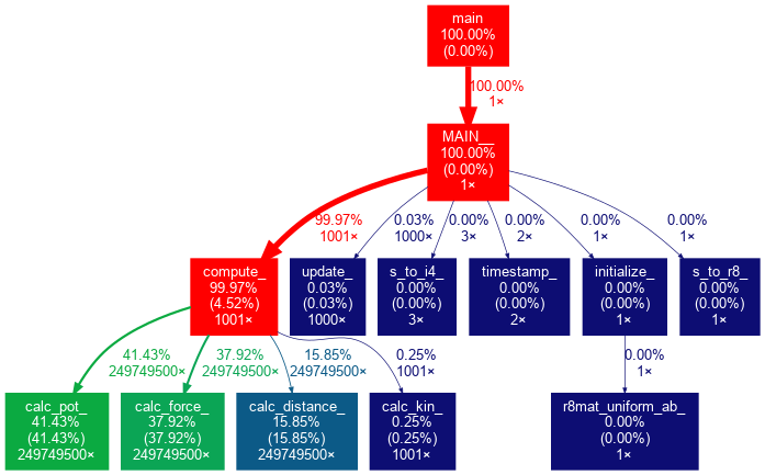
Plotting the Call Graph
The Call Graph generated by Gprof can be visualized using two tools written in Python: Gprof2Dot and GraphViz.
Install GraphViz and Gprof2Dot
These two packages need to be installed using pip.
On a production cluster you might want to create a
virtual environment
and use the --user option, like this:
$ module load python
$ virtualenv --no-download ~/Profiling_env
$ source ~/Profiling_env/bin/activate
$ pip install graphviz --no-index
$ pip install gprof2dot
On the training cluster the following is sufficient:
$ module load python
$ pip install graphviz gprof2dot
Generate the plot
The graphical representation of the call graph can be created by piping
the output of gprof into gprof2dot and it’s output further into dot
from the GraphViz package. It can be saved in different formats, e.g. PNG
(-Tpng) and under a user-defined filename (argument -o).
If a local X-server is running and X-forwarding is enabled for the current
SSH session, we can use the display command from the ImageMagick tools
to show the image. Otherwise, we can download it and display it with a program
of our choice.
$ gprof ./md_gprof  | gprof2dot -n0 -e0 | dot -Tpng -o md_gprof_graph.png
$ display md_gprof_graph.png
The call graph, visualized
Optional exercise
Create different profiles by calling the program with different parameters, e.g.
md_gprof 2 200 500 0.1andmd_gprof 2 500 1000 0.1.What doesn’t change? What does? Does that change your mind about which part of the program you should focus on first?
gprof2dot options
By default
gprof2dotwon’t display nodes and edges below a certain threshold. Because our example has only a small number of subroutines/functions, we have used the-nand-eoptions to set both thresholds to 0%.Gprof2dot has several more options to, e.g. limit the depth of the tree, show only the descendants of a function or only the ancestors of another. Different coloring schemes are available as well.
$ gprof2dot --helpUsage: gprof2dot [options] [file] ... Options: -h, --help show this help message and exit -o FILE, --output=FILE output filename [stdout] -n PERCENTAGE, --node-thres=PERCENTAGE eliminate nodes below this threshold [default: 0.5] -e PERCENTAGE, --edge-thres=PERCENTAGE eliminate edges below this threshold [default: 0.1] -f FORMAT, --format=FORMAT profile format: axe, callgrind, hprof, json, oprofile, perf, prof, pstats, sleepy, sysprof or xperf [default: prof] --total=TOTALMETHOD preferred method of calculating total time: callratios or callstacks (currently affects only perf format) [default: callratios] -c THEME, --colormap=THEME color map: color, pink, gray, bw, or print [default: color] -s, --strip strip function parameters, template parameters, and const modifiers from demangled C++ function names --colour-nodes-by-selftime colour nodes by self time, rather than by total time (sum of self and descendants) -w, --wrap wrap function names --show-samples show function samples -z ROOT, --root=ROOT prune call graph to show only descendants of specified root function -l LEAF, --leaf=LEAF prune call graph to show only ancestors of specified leaf function --depth=DEPTH prune call graph to show only descendants or ancestors until specified depth --skew=THEME_SKEW skew the colorization curve. Values < 1.0 give more variety to lower percentages. Values > 1.0 give less variety to lower percentages -p FILTER_PATHS, --path=FILTER_PATHS Filter all modules not in a specified path
Key Points
Don’t start to parallelize or optimize your code without having used a profiler first.
A programmer can easily spend many hours of work “optimizing” a part of the code which eventually speeds up the program by only a minuscule amount.
When viewing the profiler report, look for areas where the largest amounts of CPU time are spent, working your way down.
Pay special attention to areas that you didn’t expect to be slow.