Dask Array

Overview

Teaching: 15 min
Exercises: 10 min

Questions

• How can I process NumPy arrays in parallel?

• Can I distribute NumPy arrays to avoid needing all the memory on one machine?

Objectives

In the previous episode we used NumPy to speed up the computation of the mean of a large number of random numbers getting a speed up of something like 46 times. However this computation is still only done in serial, although much faster than using standard Python.

Let say we wanted to do some computation, we will stick with the mean for now, over a really large number of numbers. Lets take our script from the previous episode numpy-mean.py and adjust it a little do even more numbers. Lets also add the creation of these random numbers to our timing. Why we are adding that to our timing will become apparent shortly.

$ cp numpy-mean.py numpy-mean-lg.py
$ nano numpy-mean-lg.py

...
def main():

  #about 6G of random numbers (dim x 8 bytes/number)
  dim=50000000*16

  start=time.time()
  randomArray=np.random.normal(0.0,0.1,size=dim)
  mean=randomArray.mean()
  computeTime=elapsed(start)
...

Because we are working with so many numbers we now need some more significant memory so our srun command will have to request that.

$ srun --mem=6G python numpy-mean-lg.py

mean is 5.662568700976701e-06

==================================
compute time: 28.99828577041626s
==================================


----------------------------------------
wall clock time:29.021820068359375s
----------------------------------------

Wouldn’t it be nice if we could create and process these arrays in parallel. It turns out Dask has Arrays which work very similarly to NumPy but in parallel and optionally in a distributed way. Lets try out using Dask arrays on the above example.

$ cp numpy-mean-lg.py array-mean.py
$ nano array-mean.py

import time
import dask.array as da
...
def main():

  #about 6G of random numbers
  dim=50000000*16
  numChunks=4

  randomArray=da.random.normal(0.0,0.1,size=dim,chunks=(int(dim/numChunks)))
  meanDelayed=randomArray.mean()
  meanDelayed.visualize()

  start=time.time()
  mean=meanDelayed.compute()
  computeTime=elapsed(start)

...

Above we have replace import numpy as np with import dask.array as da and replaced np with da. The da.random.normal() call is nearly identical to the np.random.normal() call except that there is the additional parameter chunks=(<size-of-chunk>). Here we are calculating the size of the chunk based on the overall dimension of the array and how many chunks we want to create.

We have also added meanDelayed.visualize() to let us take a look at the task graph to see what Dask is doing.

Finally called the compute() function on the meanDelayed object to compute the final mean. This computation step both creates the array we are computing on using the same normal distribution and also computes the mean all with the compute() call. This is why we switched to timing both of these steps above so that we can more directly compare with the timings when using Daks array.

Now lets run it and see how we did.

$ srun --mem=7G --cpus-per-task=4 python array-mean.py&

mean is -3.506459933572822e-06

==================================
compute time: 7.353188514709473s
==================================


----------------------------------------
wall clock time:7.639941930770874s
----------------------------------------

We can take a look at the task graph that Dask created to create and calculate the mean of this 4 chunk array.

$ feh mydask.png

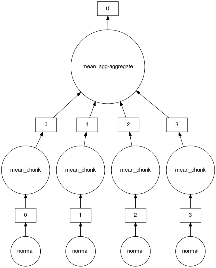
Here you can see that there are 4 tasks which create 4 array chunks from the normal distribution. These chunks are then input to the mean function which calculates the mean on each chunk. Finally a mean function which aggregates all the means of the chunks together is called to produce the final result.

Array distributed

These arrays are getting kind of big and processing them either in parallel or in serial on a single compute node restricts us to nodes that have more than about 7G of memory. Now on real clusters 7G of memory isn’t too bad but if arrays get bigger this could easily start to restrict how many of the nodes on the clusters you can run your jobs on to only the fewer more expensive large memory nodes. However, Dask is already processing our arrays in separate chunks on the same node couldn’t we distributed it across multiple nodes and reduce our memory requirement for an individual node?

If we wanted to be able to run on computations of large arrays with less memory per compute node could we distributed these computations across multiple nodes? Yes we can using the distributed computing method we saw earlier.

Solution

Start with the array-mean.py script we just created and add to it the distributed Dask cluster creation code.

$ cp array-mean.py array-distributed-mean.py
$ nano array-distributed-mean.py

import time
import dask.array as da
from dask_jobqueue import SLURMCluster
from dask.distributed import Client
...
def main():
...
  #memory=6G data / 16chunks x 4 cores per worker =1.5G plus a little extra
  cluster=SLURMCluster(cores=1,memory="2G",walltime='00:05:00')
  client=Client(cluster)
  cluster.scale(numWorkers)
  time.sleep(5)

  start=time.time()
  mean=meanDelayed.compute()
  computeTime=elapsed(start)

  client.close()
  cluster.close()
...

array-distributed-mean.py

$ srun python array-distributed-mean.py&
$ sqcm

  JOBID PARTITION     NAME   USER ST  TIME NODES CPUS MIN_M NODELIST
   1748 cpubase_b   python user49  R  0:05     1    1  256M node-sml1
   1749 cpubase_b dask-wor user49  R  0:01     1    1    2G node-sml1
   1750 cpubase_b dask-wor user49  R  0:01     1    1    2G node-sml2
   1751 cpubase_b dask-wor user49  R  0:01     1    1    2G node-mdm1
   1752 cpubase_b dask-wor user49  R  0:01     1    1    2G node-mdm1

Each of our workers is only using 2G of memory. While overall we are using 8G+256M of memory each compute node only has to have 2G of memory available, not the whole 7G on a single node that we needed for the serial or multi-threaded processing we did previously.

mean is -1.0935938328889444e-06

==================================
compute time: 9.609684467315674s
==================================


----------------------------------------
wall clock time:16.987823486328125s
----------------------------------------

It took a little longer to do the computation than it did when the computing happened all on the same node and there was extra time to create the cluster and wait for it to spin up, but it did allow us to do our computation with less memory per node and that can be very valuable in getting your job through the work queue faster on a production system as large memory nodes are few and very sought after.

Key Points