Introduction

Overview

Teaching: 15 min
Exercises: 0 min

Questions

What is Dask?

How does it work?

Objectives

Dask is a flexible library for parallel computing in Python. Python code is (or was) a bit notoriously difficult to parallelize because of something called the global interpreter lock (GIL) which essentially meant Python couldn’t be multi-threaded within a single process. Dask was started because of a desire to parallelize the existing SciPy stack and libraries spun off from that. It started by attempting to parallelize the NumPY library because it forms the basis on which SciPy was built. NumPy was also difficult to use when working with large datasets that didn’t fit nicely into memory but that fit nicely onto disk.

Dask tries to be familiar

If you are already used to working with python module such as NumPy, Pandas, or PySpark Dask provides similar interfaces allowing python code already using these modules to be converted to use Dask parallel constructs easily.

How does Dask work?

Dask creates task graphs

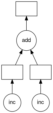
Dask creates a graph of tasks, which show the inter-dependencies of the tasks. These tasks are usually functions that operate on some input. Below is an example of a very basic visualization of one of these task graphs for a particular set of tasks. The circles represent the function and the arrows point from the function to boxes which represent the output of the function. These outputs then have arrows which point to further functions which use these outputs as inputs.

Dask task graph

Dask schedules tasks

With the task graph in hand, Dask will schedule tasks on workers/threads and ensure the outputs of those tasks get from one task to the next in the graph. There are a number of different ways Dask can schedule these tasks from serial, to multi-threaded, to across multiple distributed compute nodes on an HPC cluster.

Dask task graph compute flow

Beginnings of Dask

Dask is a fairly new project. The First commit to the Dask project occurred in Dec, 2014. Dask started small, see how short the first commit is. The core.py file is only 21 lines including white space. If you look at the test_comprehensive_user_experience function you can see how it was to be used very early on. It already looked a lot like Dask Delayed does now, as we shall see.

In this test function it records the functions inc and add and their arguments and then later executes those calculations using the get function to produce the final result of the calculation.

Key Points

Python

Overview

Teaching: 25 min
Exercises: 0 min

Questions

What is a virtual environment?

How can you time Python scripts?

What is a simple way to run a Python script on a compute node?

Objectives

Before we get to working with Dask we need to setup our Python environment, some basic timing of python code, and create a script that does something slightly interesting that we can use as a starting point to work with Dask.

Virtual environment setup

Connect to the server using your own username and check to see if your x11 forwarding is working.

$ ssh -X <your-username>@pcs.ace-net.training
$ xclock

You should now be connected to the training cluster and hopefully if you have an x11 server running you should see a little analog clock pop up in a window. If you can’t get x11 forwarding working, it isn’t the end of the world. There is one small exercise where you will have look at the solution to see the graph rather than viewing the image yourself.

Next load the Python module.

$ module load python

There is a version of python already available on the login node, but for consistency between clusters it is better to use the python version available through module system. If we wanted we could specify a particular version of the Python module to load, with something like module load python/3.8.10. For more information about using modules see the Alliance documentation on modules.

Next lets create a python virtual environment for our dask work and activate it.

$ virtualenv --no-download dask
$ source ~/dask/bin/activate

A Python virtual environment provides an isolated place to install different Python packages. You can create multiple virtual environments to install different packages or versions of packages and switch between them to keeping each environment separate from each other avoiding version conflicts. For more information about using virtual environments see the Alliance documentation on python virtual environments.

Running a Python script

Lets create a basic “hello world” python script and make sure we can run it as a starting point.

$ nano hello.py

This starts the nano editor, editing a new file hello.py.

Lets create our first python script just to check that we have everything working. In the editor add the following code.

def main():
  print("hello world")

if __name__=="__main__":
  main()

Save and exit by pressing ‘ctrl’+’x’ answering ‘y’ when asked if you would like to save followed by pressing enter to accept the filename.

This is a pretty standard way to create a Python script so that if you import it as a module the main function isn’t executed but you can access all the functions defined in it. However if you run it on the command line the main function will be executed.

Lets run the script to see if everything is working.

$ python ./hello.py

hello world

Timing

Since we are going to be parellelizing code using Dask it is useful to see what effect our efforts have on the run time. Lets add some code to our hello.py script to time execution.

$ nano hello.py

import time

def elapsed(start):
  return str(time.time()-start)+"s"
def main():
  print("hello world")

if __name__=="__main__":
  start=time.time()
  main()
  wallClock=elapsed(start)
  print()
  print("----------------------------------------")
  print("wall clock time:"+wallClock)
  print("----------------------------------------")
  print()

hello.py

$ python hello.py

hello world

----------------------------------------
wall clock time:2.574920654296875e-05s
----------------------------------------

Running on a compute node

Next to run more computationally intensive scripts or to run with multiple cores it is best to run the job on a compute node. To run on a compute node the srun command can be used.

$ srun python hello.py

hello world

----------------------------------------
wall clock time:7.867813110351562e-06s
----------------------------------------

This command runs our script on a compute node granting access to a single compute core. The srun command is perfect in this training environment but there other, likely better, ways to run the Alliance HPC clusters, for more info see the Alliances documentation on running jobs.

A more interesting script

To let us see how Dask can be used to parallelize a python script lets first write a bit more interesting python script to parallelize with Dask in the next episode.

$ cp ./hello.py pre-dask.py
$ nano pre-dask.py

import time

def elapsed(start):
  return str(time.time()-start)+"s"

def inc(x):
  time.sleep(1)
  return x+1
def add(x,y):
  time.sleep(1)
  return x+y

def main():
  x=inc(1)
  y=inc(2)
  z=add(x,y)
  print("z="+str(z))

if __name__=="__main__":
  start=time.time()
  main()
  wallClock=elapsed(start)
  print()
  print("----------------------------------------")
  print("wall clock time:"+wallClock)
  print("----------------------------------------")
  print()

pre-dask.py

Save and exit and run on a compute node with the following command and take note of the runtime.

$ srun python ./pre-dask.py

z=5

----------------------------------------
wall clock time:3.0034890174865723s
----------------------------------------

It takes about 3s which isn’t too surprising since we have three function calls all with a 1s sleep in them. Clearly this sleep is dominating the run time. This is obviously artificial but will allows us to have a well understood compute requirements while we are exploring Dask.

Key Points

Dask Delayed

Overview

Teaching: 20 min
Exercises: 20 min

Questions

How do you install Dask Delayed?

How can Dask Delayed be used to parallelize python code?

How can I see what Dask Delayed is doing?

Objectives

Installing Dask

Before we can use dask we must install it with the following command on the terminal.

$ pip install pandas numpy dask distributed graphviz bokeh dask_jobqueue mimesis requests matplotlib

This actually installs lots of stuff, not just Dask, but should take around 2 minutes or a bit less. This will install these modules into the virtual environment we setup and are currently working in.

Using Dask Delayed

Lets start by looking at the python code we have from the last episode and thinking about what parts could be run in parallel.

import time

def elapsed(start):
  return str(time.time()-start)+"s"

def inc(x):
  time.sleep(1)
  return x+1
def add(x,y):
  time.sleep(1)
  return x+y

def main():
  x=inc(1)
  y=inc(2)
  z=add(x,y)
  print("z="+str(z))

if __name__=="__main__":
  start=time.time()
  main()
  wallClock=elapsed(start)
  print()
  print("----------------------------------------")
  print("wall clock time:"+wallClock)
  print("----------------------------------------")
  print()

pre-dask.py

The two calls to the inc functions could be called in parallel, because they are totally independent of one-another.

We can use dask.delayed on our functions to make them lazy. When we say lazy we mean that those functions will not be called immediately. What happens instead is that it records what we want to compute as a task into a graph that we will run later using the compute member function on the object returned by the dask.delayed function.

Lets add the new Dask code now.

$ cp pre-dask.py delayed.py
$ nano delayed.py

import time
import dask

...

def main():
  x=dask.delayed(inc)(1)
  y=dask.delayed(inc)(2)
  z=dask.delayed(add)(x,y)
  #result=z.compute()
  #print("result="+str(result))
  
...

However, to illustrate that nothing happens until z.compute() is called lets comment it and the following print line out and run it.

$ srun python ./delayed.py

----------------------------------------
wall clock time:0.22939133644104004s
----------------------------------------

It clearly didn’t call our inc or add functions as any one of those calls should take at least 1 s and the total time is well below 1s. Now lets uncomment the code and rerun it.

...

def main():
  ...
  z=dask.delayed(add)(x,y)
  result=z.compute()
  print("result="+str(result))
...

delayed.py

$ srun python ./delayed.py

result=5

----------------------------------------
wall clock time:3.3499603271484375s
----------------------------------------

Hey, that’s no faster than the non-dask version. In fact it is a very tiny bit slower. What gives? Well, we only ran it on one core. Lets try on two cores and see what happens.

$ srun --cpus-per-task=2 python ./delayed.py

result=5

----------------------------------------
wall clock time:2.169353485107422s
----------------------------------------

Ah that’s better it is now down to about 2s from our original 3s. To help us understand what Dask is doing we can use the member function visualize of the Delayed object which creates a visualization of the graph Dask created for our tasks.

...
def main():
  ...
  z=dask.delayed(add)(x,y)
  z.visualize()
  #result=z.compute()
  #print("result="+str(result))
...

$ srun python ./delayed.py

Which returns fairly quickly because we aren’t actually doing any work. However it has created a mydask.png file which lets us visualize what Dask will do. Lets have a look at it (this requires the -X option to work and a x11 server running).

$ feh mydask.png

Notice that this includes the names of the functions from our script and the logical flow of the outputs from the inc function to the inputs of the add function.

Here you can see that the two inc functions can be run in parallel provided we have hardware capable of running them at the same time and afterwards the add function will be run in serial.

Parallelize a loop

Download the below script with the below wget command.

$ wget https://raw.githubusercontent.com/acenet-arc/ACENET_Summer_School_Dask/gh-pages/code/loop-template.py

import time

def elapsed(start):
  return str(time.time()-start)+"s"

def inc(x):
  time.sleep(1)
  return x+1
def main():
  data=[1,2,3,4,5,6,7,8]
  dataInc=[]
  for x in data:
    y=inc(x)
    dataInc.append(y)
  total=sum(dataInc)
  print("total="+str(total))
  
if __name__=="__main__":
  start=time.time()
  main()
  wallClock=elapsed(start)
  print()
  print("----------------------------------------")
  print("wall clock time:"+wallClock)
  print("----------------------------------------")
  print()

loop-template.py

Run this script to with --cpus-per-task=1 and note the run time.

Then apply what you have learned to parallelize this script. Then run with --cpus-per-task=1,2, and 4 and note the times.

Solution

import time
import dask
...
def main():
  ...
  for x in data:
    y=dask.delayed(inc)(x)
    dataInc.append(y)
  total=dask.delayed(sum)(dataInc)
  result=total.compute()
  print("total="+str(result))
...

loop-solution.py

Serial

srun --cpus-per-task=1 python loop-template.py

total=44

----------------------------------------
wall clock time:8.008957147598267s
----------------------------------------

Delayed Serial

srun --cpus-per-task=1 python loop-solution.py

total=44

----------------------------------------
wall clock time:8.009050607681274s
----------------------------------------

Delayed 2 CPUs

srun --cpus-per-task=2 python loop-solution.py

total=44

----------------------------------------
wall clock time:4.008902311325073s
----------------------------------------

Delayed 4 CPUs

srun --cpus-per-task=4 python loop-solution.py

total=44

----------------------------------------
wall clock time:2.005645990371704s
----------------------------------------

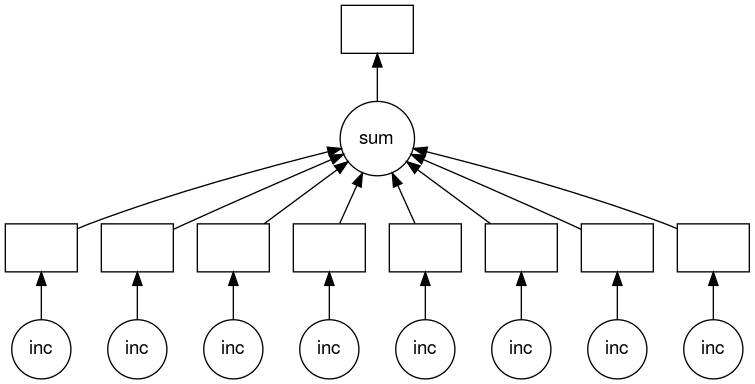
Visualize loop parallelization

Use the solution to the previous challenge to visualize how the loop is being parallelized by Dask.

You can get the solution with the following command.
$ wget https://raw.githubusercontent.com/acenet-arc/ACENET_Summer_School_Dask/gh-pages/code/loop-solution.py
Solution
...
def main():
  ...
  total=dask.delayed(sum)(dataInc)
  total.visualize()
  result=total.compute()
  ...
$ srun --cpus-per-task=4 python loop-solution.py
$ feh mydask.png

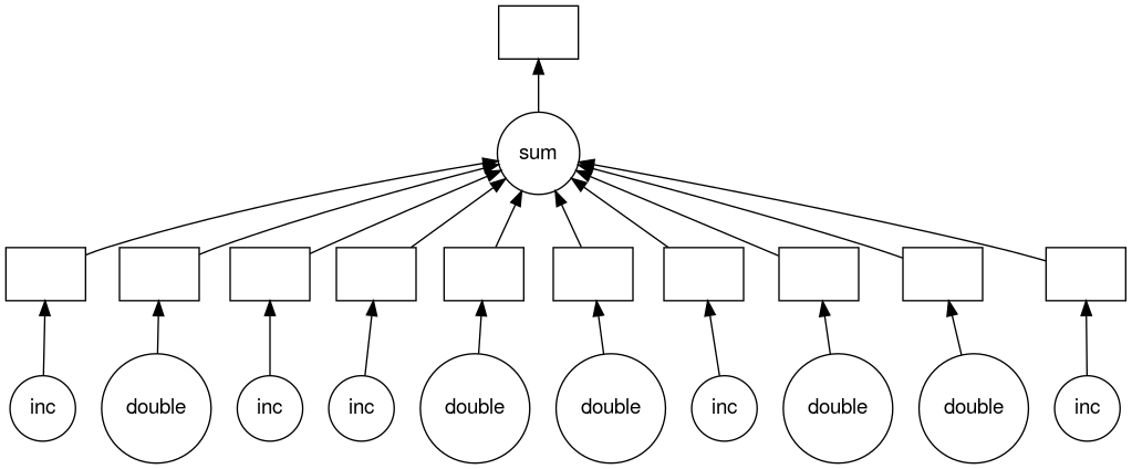
Parallelize loop with flow control

Download the below script with the below wget command.

$ wget https://raw.githubusercontent.com/acenet-arc/ACENET_Summer_School_Dask/gh-pages/code/loop-flow-template.py

import time

def inc(x):
  time.sleep(1)
  return x+1
def double(x):
  time.sleep(1)
  return 2*x
def isEven(x):
  return not x % 2
def main():
  data=[1,2,3,4,5,6,7,8,9,10]
  dataProc=[]
  for x in data:
    if isEven(x):
      y=double(x)
    else:
      y=inc(x)
    dataProc.append(y)

  total=sum(dataProc)
  print("total="+str(total))
if __name__=="__main__":
  start=time.time()
  main()
  end=time.time()
  print("wall clock time:"+str(end-start)+"s")

loop-flow-template.py

Then parallelize with dask.delayed, compute, and visualize the task graph.

Solution

import time
import dask
...
def main():
  ...
  for x in data:
    if isEven(x):
      y=dask.delayed(double)(x)
    else:
      y=dask.delayed(inc)(x)
    dataProc.append(y)

  total=dask.delayed(sum)(dataProc)
  total.visualize()
  result=total.compute()
  ...

loop-flow-solution.py

Loop with flow control parallelization graph

Key Points

Break

Overview

Teaching: min
Exercises: min

Questions

Objectives

Key Points

Real Computations

Overview

Teaching: 15 min
Exercises: 10 min

Questions

What happens when I use Dask for “real” computations?

How can I see CPU efficiency of a SLURM Job?

Objectives

So far we have seen how to use Dask delayed to speed up or parallelize the time.sleep() function. Lets now try it with some “real” computations.

Lets start with our hello.py script and add some functions that do some computations and used Dask delayed to parallelize them.

$ cp hello.py compute.py
$ nano compute.py

Then edit to contain the following.

import time
import dask

def elapsed(start):
  return str(time.time()-start)+"s"

def computePart(size):
  part=0
  for i in range(size):
    part=part+i
  return part

def main():

  size=40000000
  numParts=4

  parts=[]
  for i in range(numParts):
    part=dask.delayed(computePart)(size)
    parts.append(part)
  sumParts=dask.delayed(sum)(parts)

  start=time.time()
  sumParts.compute()
  computeTime=elapsed(start)

  print()
  print("=======================================")
  print("Compute time: "+computeTime)
  print("=======================================")
  print()

if __name__=="__main__":
  start=time.time()
  main()
  wallClock=elapsed(start)
  print()
  print("----------------------------------------")
  print("wall clock time:"+wallClock)
  print("----------------------------------------")
  print()

compute.py

Lets run it.

$ srun --cpus-per-task=1 python compute.py

=======================================
Compute time: 11.632155656814575s
=======================================


----------------------------------------
wall clock time:11.632789134979248s
----------------------------------------

More cores!

Take the compute.py code and run it with different numbers of cores like we did for the delayed.py code. What do you expect to happen? What actually happens?

Solution

1 core

$ srun --cpus-per-task=1 python compute.py

=======================================
Compute time: 11.632155656814575s
=======================================


----------------------------------------
wall clock time:11.632789134979248s
----------------------------------------

2 cores

$ srun --cpus-per-task=2 python compute.py

=======================================
Compute time: 11.144386768341064s
=======================================


----------------------------------------
wall clock time:11.14497971534729s
----------------------------------------

4 cores

$ srun --cpus-per-task=4 python compute.py

=======================================
Compute time: 11.241060972213745s
=======================================


----------------------------------------
wall clock time:11.241632223129272s
----------------------------------------

Shouldn’t they be approximately dividing up the work, but the times are all about the same?

In the last exercise we learned that our “computations” do not parallelize as well as the time.sleep() function did previously. To explore this lets take a look at the CPU efficiency of our jobs. To do this we can use the seff command which outputs stats for a job after it has completed given the JobID including the CPU efficiency. But where do we get the JobID? To get the JobID we can run our jobs in the background by appending the & character to our srun command. Once we have our job running in the background we check on it in the queue to get the JobID.

To make it a little easier to see what is going on in our queue lets create an alias for the squeue command with some extra options.

$ alias sqcm="squeue -u $USER -o'%.7i %.9P %.8j %.7u %.2t %.5M %.5D %.4C %.5m %N'"

Now we can run the command sqcm and get only our jobs (not everyones) and also additional information about our jobs, for example how many cores and how much memory was requested.

Lets run a job now and try it out.

$ srun --cpus-per-task=1 python compute.py&
$ sqcm

 JOBID PARTITION     NAME   USER ST  TIME NODES CPUS MIN_M NODELIST
    964 cpubase_b   python user49  R  0:10     1    1  256M node-mdm1
$
=======================================
Compute time: 11.121154069900513s
=======================================


----------------------------------------
wall clock time:11.121747255325317s
----------------------------------------

I got the output from our sqcm command followed a little later by the output of our job. It is important to run the sqcm command before the job completes or you won’t get to see the JobID.

Our sqcm command showed us that our job was running with one CPU on one node and with 256M of memory. It also shows us how long the job has run for and let us see the JobID.

When the srun command is running in the background I found I had to press the return key to get my prompt back and at the same time got a message about my background srun job completing.

[1]+  Done                    srun --cpus-per-task=1 python compute.py
$

With the JobID we can use the seff command to see what the cpu efficiency was.

$ seff 965

Job ID: 965
Cluster: pcs
User/Group: user49/user49
State: COMPLETED (exit code 0)
Cores: 1
CPU Utilized: 00:00:11
CPU Efficiency: 84.62% of 00:00:13 core-walltime
Job Wall-clock time: 00:00:13
Memory Utilized: 0.00 MB (estimated maximum)
Memory Efficiency: 0.00% of 256.00 MB (256.00 MB/core)

We got almost 85% CPU efficiency, not too bad.

CPU efficiency

Given what we just learned about how to check on a jobs efficiency, lets re-run our dask jobs with different numbers of cores 1,2,4 and see what the CPU efficiency is.

Solution

1 core

$ srun --cpus-per-task=1 python compute.py&
$ sqcm

  JOBID PARTITION     NAME   USER ST  TIME NODES CPUS MIN_M NODELIST
    966 cpubase_b   python user49  R  0:04     1    1  256M node-mdm1

$ seff 966

Job ID: 966
Cluster: pcs
User/Group: user49/user49
State: COMPLETED (exit code 0)
Cores: 1
CPU Utilized: 00:00:11
CPU Efficiency: 91.67% of 00:00:12 core-walltime
Job Wall-clock time: 00:00:12
Memory Utilized: 0.00 MB (estimated maximum)
Memory Efficiency: 0.00% of 256.00 MB (256.00 MB/core)

2 cores

$ srun --cpus-per-task=2 python compute.py&
$ sqcm

  JOBID PARTITION     NAME   USER ST  TIME NODES CPUS MIN_M NODELIST
    967 cpubase_b   python user49  R  0:04     1    2  256M node-mdm1

$ seff 967

Job ID: 967
Cluster: pcs
User/Group: user49/user49
State: COMPLETED (exit code 0)
Nodes: 1
Cores per node: 2
CPU Utilized: 00:00:12
CPU Efficiency: 50.00% of 00:00:24 core-walltime
Job Wall-clock time: 00:00:12
Memory Utilized: 12.00 KB
Memory Efficiency: 0.00% of 512.00 MB

4 cores

$ srun --cpus-per-task=4 python compute.py&
$ sqcm

  JOBID PARTITION     NAME   USER ST  TIME NODES CPUS MIN_M NODELIST
    968 cpubase_b   python user49  R  0:04     1    4  256M node-mdm1

$ seff 968

Job ID: 968
Cluster: pcs
User/Group: user49/user49
State: COMPLETED (exit code 0)
Nodes: 1
Cores per node: 4
CPU Utilized: 00:00:12
CPU Efficiency: 25.00% of 00:00:48 core-walltime
Job Wall-clock time: 00:00:12
Memory Utilized: 4.00 KB
Memory Efficiency: 0.00% of 1.00 GB

The efficiencies are ~ 92%, 50%, and 25% for 1,2,4 CPUs respectively. It looks like very little if any of these threads are running in parallel.

What is going on, where did our parallelism go? Remember the Global Interpreter Lock (GIL) I mentioned way back at the beginning? Well that’s what is going on! When a thread needs to use the Python interpreter it locks access to the interpreter so no other thread can access it, when it is done it releases the lock and another thread can use it. This means that no single thread can execute Python code at the same time!

But why did our sleep function work? When we used the sleep function, the waiting happens outside the Python interpreter. In this case each thread will happily wait in parallel since the ‘work’ inside the sleep function doesn’t have to wait for the Python interpreter to become free and so they can run in parallel. This goes for any other function calls that do not run in the Python interpreter, for example NumPy operations often run as well-optimized C code and don’t need the Python interpreter to operate, however it can be tricky to know exactly when and how the Python interpreter will be needed.

Does this mean Dask is not that great for parallelism? Well, the way we have used it so far can be useful in certain circumstances, for example what I mentioned about NumPy above, however there is another way you can use Dask, and that is in a distributed way. Lets look at that now!

Key Points

Lunch Break

Overview

Teaching: min
Exercises: min

Questions

Objectives

Key Points

Distributed Computations

Overview

Teaching: 25 min
Exercises: 15 min

Questions

How can I avoid the GIL problem?

How can I run multiple Python interpreters at once on one problem?

Objectives

So we have started to see some of the implications of GIL when we are using Dask. Now we will look at a way to avoid it even if your code needs frequent access to the Python Interpreter (e.g. you haven’t converted a bunch of it to C code with something like Cython which can seriously improve the performance of Python code even before parallelization).

The basic idea with distributed computations is to give each execution of your Python code it’s own Python interpreter. This means that there will necessarily be massage passing and coordinating between the different processes running the different Python interpreters. Luckily Dask takes care of all this for us and after a bit of additional setup we can use it with Delayed just as we did before but without issues with GIL.

Since we are coming back from last day we have to log back into the cluster and re-activate our virtual environment.

$ ssh -X <your-username>@pcs.ace-net.training
$ source ~/dask/bin/activate

Lets also re-do our squeue alias as we will want that. To make this permanent you could put this line into your ~/.bashrc file.

$ alias sqcm="squeue -u $USER -o'%.7i %.9P %.8j %.7u %.2t %.5M %.5D %.4C %.5m %N'"

Lets start with our previous compute.py script and modify it to run in a distributed way.

$ cp compute.py compute-distributed.py
$ nano compute-distributed.py

import time
import dask
from dask_jobqueue import SLURMCluster
from dask.distributed import Client
...
def main():

  size=40000000
  numParts=4
  numWorkers=1

  parts=[]
  for i in range(numParts):
    part=dask.delayed(computePart)(size)
    parts.append(part)
  sumParts=dask.delayed(sum)(parts)

  #create the "cluster"
  cluster=SLURMCluster(cores=1,memory="256M",walltime='00:05:00')

  #Show us the job script used to launch the workers
  print(cluster.job_script())
  client=Client(cluster)

  #create the workers
  cluster.scale(numWorkers)

  #sleep a little bit for workers to create and
  #check in with the scheduler
  time.sleep(5)

  start=time.time()
  sumParts.compute()
  computeTime=elapsed(start)

  client.close()
  cluster.close()
...

compute-distributed.py

In the above script we have added a few bits. We have imported SLURMCluster which allows us to submit jobs to create independent Dask workers and we have imported the Dask Client so that we can tell it to use the software Dask cluster we create.

We can create some number of workers using the cluster.scale(numWorkers) function. After these setup bits our computation continues as normal with Dask Delayed.

Lets run our new script, this time the computation is all done in the workers and not in the job we submit with the srun command. There is no need to change the number of CPUs we request as that is all taken care of by changing the numWorkers variable. Lets also immediately run the sqcm command to see what jobs we have running and frequently afterwards to see how Dask spawns new workers for us.

$ srun python compute-distributed.py&
$ sqcm

  JOBID PARTITION     NAME   USER ST  TIME NODES CPUS MIN_M NODELIST
    980 cpubase_b   python user49  R  0:02     1    1  256M node-mdm1

Here you can just see our first job we submitted.

$ sqcm

  JOBID PARTITION     NAME   USER ST  TIME NODES CPUS MIN_M NODELIST
    981 cpubase_b dask-wor user49 PD  0:00     1    1  245M
    980 cpubase_b   python user49  R  0:04     1    1  256M node-mdm1

Here you can see the worker job that Dask spawned for our work is in the PD or pending state.

$ sqcm

  JOBID PARTITION     NAME   USER ST  TIME NODES CPUS MIN_M NODELIST
    980 cpubase_b   python user49  R  0:07     1    1  256M node-mdm1
    981 cpubase_b dask-wor user49  R  0:02     1    1  245M node-mdm1

Finally here we see that the worker is up and running.

#SBATCH -J dask-worker
#SBATCH -n 1
#SBATCH --cpus-per-task=1
#SBATCH --mem=245M
#SBATCH -t 00:05:00

/home/user49/dask/bin/python -m distributed.cli.dask_worker tcp://192.168.0.133:44075 --nthreads 1 --memory-limit 244.14MiB --name dummy-name --nanny --death-timeout 60

Above we see a print out of the job script that Dask uses to launch our workers. The settings for this script come from the settings we gave to the SLURMCluster function.

=======================================
Compute time: 12.071980953216553s
=======================================


----------------------------------------
wall clock time:18.724435329437256s
----------------------------------------

And finally we get our timings for performing our computations. A little longer than with our pur Dask Delayed code, but lets see how it changes with more cores, or rather more workers.

More cores distributed

Given the above compute-distributed.py run first with numWorkers=1 to get a base line, then run with numWorkers=2, 4, and 8.

HINT: you don’t need to change the srun python compute-distributed.py& command as you change the number of workers.
Solution

numWorkers=1
====================================
Compute time: 12.333828449249268s
====================================
numWorkers=2
====================================
Compute time= 6.07476544380188s
====================================
numWorkers=4
====================================
Compute time= 3.454866409301758s
====================================
numWorkers=8
====================================
Compute time= 3.3805696964263916s
====================================
Now we are getting some true parallelism. Notice how more than 4 workers doesn’t improve things, why is that?

Running on busy clusters

In this workshop we have been learning about Dask on a relatively quite training cluster. On a production cluster creating a job which then creates other worker jobs to perform computations might not be the best option as it could take quite some time for the worker jobs to start up and connect to the managing job. This time for worker jobs to start up may exceed the original job’s time limit. A possible alternative could be to use Dask-MPI to launch all workers inside a single MPI job.

Key Points

Cython

Overview

Teaching: 30 min
Exercises: 10 min

Questions

How slow is Python?

Can I make my Python code faster?

How can I turn my Python code into compiled C or C++ code?

Objectives

Python is built for the programmer not the computer. What do I mean by that? Python is a very nice programming language to program in. You can get your ideas and algorithms written out very quickly as the Python language manages a lot of the aspects of memory management for you and provides convenient and flexible data structures that just work the way you expect them to without much effort on the part of the programmer to get it right. Part of this comes from the fact that Python is “duck” typed. Meaning, if a Python object looks like a duck, quacks like a duck, it is a duck. This means that you can pass different types of objects to a function and as long as that function can access the member functions of that object that it needs to work with it doesn’t care what type of object you passed it. This allows you to write code faster and greatly increases the flexibility and re-usability of your Python code. However, you pay for these benefits with your program run times.

If you are are not doing any heavy computing this might be just fine, perhaps your CPUs wouldn’t be doing that much work anyhow, and waiting another second to get your work done more than offsets the extra hours or days it might take you to write your algorithm out in another language like C or Fortran. However, if you are doing numerically intensive programming this can become a serious problem and is part of the reason most computationally intensive programs aren’t written in Python.

One common solution to this problem is to take the parts of your Python program that are computational intensive and convert them to a compiled language that is much faster. One really nice thing about Python is how well integrated it is with C and C++.

You can extend python with C or C++ by writing modules that you can import and use in your Python scripts. This however does take a bit of doing. Most of the extra effort involves creating the interfaces and Python objects to go between the C or C++ code and the Python scripts. For more details about how to do this see these Python docs on extending Python with C or C++.

You can also embed Python in a C or C++ application allowing it to call your Python functions from inside that application. This can be very handy for allowing scripting support within applications. For more details about embedding Python in C or C++ applications check these Python docs on embedding Python in another application.

These two approaches are powerful, but do involve being very proficient at C and C++ and take a bit of doing to get working correctly. Though they provide the programmer with a lot of control in how the C or C++ portions of the application interface with the Python portions. If you are willing to give up some of this control for a short cut Cython is a good compromise.

Cython helps you compile your Python code into C code so that you can get the performance benefits of a compiled language without having to do too much extra work to get there. But before we get too far into Cython, lets install it so it is ready to go.

$ pip install cython

Now that Cython is installed lets take a look at how we can use it.

In Python you can declare a variable as below.

x=0.5

You don’t have to tell Python anything about the type of variable. In Python everything is an object (even floats and integers). This makes them super flexible but also more computationally and memory intensive.

One of the big differences in most compiled languages, and certainly is the case in both C and C++, is that every variable must be declared with a specific type. This means that at compile time the compiler has enough information about how something is going to work to perform more optimizations when generating the machine code that you will ultimately be running. In addition, if your floating point variable has a lot of extra baggage associated with it because it is actually a more complicated object, it can also increase memory requirements, which has impacts on performance as it might not fit as neatly into a cache line.

To allow Cython to generate compilable C and C++ code from our Python code we need to add some extra information about the types of our variables.

Some examples of how to do this with Cython is shown below.

cdef int a,b,c
cdef char *s
cdef float x=0.5
cdef double x=63.4
cdef list names

We also need to provide information about the return types and parameters of our functions and weather these functions will be called only from within the converted C code, cdef, or only from Python, def, or both, cpdef.

def test(x): #regular python function, calls from Python only
  ...
cdef int test(float x): #Cython only functions which can't be accessed from Python-only code.
  ...
cpdef int test2(float x, double y): #Can be accessed from either Cython or Python code.
  ...

Notice how the C/C++ variable types are showing up here as int the return type of the functions and the float or double types given for the function parameters.

Lets try this out in a full example.

$ cp hello.py dosum.py
$ nano dosum.py

...
def sumnum(n):
  result=0.0
  for i in range(n):
    result+=float(i)
  return result
def main():
  size=40000000
  start=time.time()
  result=sumnum(size)
  computeTime=elapsed(start)
  print("result="+str(result)+" computed in "+str(computeTime))
...

dosum.py

Lets quickly test it to make sure it works properly.

$ srun python dosum.py

result=799999980000000.0 computed in 5.351787805557251s

----------------------------------------
wall clock time:5.352024793624878s
----------------------------------------

In preparation for speeding up our sumnum function with Cython lets pull it out into a separate Python module.

$ nano pysum.py

def sumnum(n):
  result=0.0
  for i in range(n):
    result+=float(i)
  return result

pysum.py

Now copy and modify our original script to use our sumnum function from the newly created Python module and remove our old version of the sumnum function from the driver script.

$ cp dosum.py dosum_driver.py
$ nano dosum_driver.py

import time
import pysum
...
def main():
  size=40000000
  start=time.time()
  result=pysum.sumnum(size)
  computeTime=elapsed(start)
  print("result="+str(result)+" computed in "+str(computeTime))
...

Verify everything still works.

$ srun python dosum_driver.py

result=799999980000000.0 computed in 5.351787805557251s

----------------------------------------
wall clock time:5.352024793624878s
----------------------------------------

Looks good. Now lets create a Cython version of our pysum.py module adding in the type declarations as mentioned previously.

$ cp pysum.py cysum.pyx
$ nano cysum.pyx

cpdef double sumnum(int n):
  cdef double result=0.0
  cdef int i
  for i in range(n):
    result+=i
  return result

cysum.pyx

Next create a build_cysum.py file which will act like a Makefile for compiling our cysum.pyx script.

$ nano build_cysum.py

from distutils.core import setup
from Cython.Build import cythonize

setup(ext_modules=cythonize('cysum.pyx'))

build_cysum.py

Then compile our Cython code with the following command.

$ python build_cysum.py build_ext --inplace

Finally lets modify our driver script to use our newly created Cython version of the sumnum function and compare it to the old version.

$ nano dosum_driver.py

import time
import pysum
import cysum
...
def main():
  size=40000000
  
  start=time.time()
  result=pysum.sumnum(size)
  computeTime=elapsed(start)
  print("pysum result="+str(result)+" computed in "+str(computeTime))
  
  start=time.time()
  result=cysum.sumnum(size)
  computeTime=elapsed(start)
  print("cysum result="+str(result)+" computed in "+str(computeTime))
...

dosum_driver.py

$ srun python dosum_driver.py

pysum result=799999980000000.0 computed in 5.7572033405303955s
cysum result=799999980000000.0 computed in 0.11868977546691895s

----------------------------------------
wall clock time:5.876289129257202s
----------------------------------------

Ok, so our Cython version is much faster, 5.75/0.12=47.91, so nearly 48 times faster. That’s a pretty nice speed up for not a lot of work.

Cythonize our compute-distributed.py script

In the previous episode we had created a script that parallelized our computePart function across multiple distributed Dask workers. Lets now Cythonize that function to improve our performance even further to see if we can get below that approximately 3.4s of compute time when running with 4 workers having one core each.

If you need a copy of that script you can download it with:
$ wget https://raw.githubusercontent.com/acenet-arc/ACENET_Summer_School_Dask/gh-pages/code/compute-distributed.py
Solution

Create a new module file containing our computePart function and “Cythonize” it.
$ nano computePartMod.pyx
cpdef int computePart(int size):
  cdef int part=0
  cdef int i
  for i in range(size):
    part=part+i
  return part
computePartMod.pyx
Next create our file describing how we want to build our Cython module for the computePart function.
$ nano build_computePartMod.py
from distutils.core import setup
from Cython.Build import cythonize

setup(ext_modules=cythonize('computePartMod.pyx'))
build_computePartMod.py
Then compile it.
$ python build_computePartMod.py build_ext --inplace
Finally import our newly cythonized module and call the computePart function from it.
$ cp compute-distributed.py compute-distributed-cython.py
$ nano compute-distributed-cython.py
import time
import dask
from dask_jobqueue import SLURMCluster
from dask.distributed import Client
import computePartMod
...
def main():

  size=40000000
  numParts=4
  numWorkers=4

  parts=[]
  for i in range(numParts):
    part=dask.delayed(computePartMod.computePart)(size)
...
compute-distributed-cython.py
Lets see the results.
$ srun python compute-distributed-cython.py
#!/usr/bin/env bash

#SBATCH -J dask-worker
#SBATCH -n 1
#SBATCH --cpus-per-task=1
#SBATCH --mem=245M
#SBATCH -t 00:05:00

/home/user49/dask/bin/python -m distributed.cli.dask_worker tcp://192.168.0.222:35157 --nthreads 1 --memory-limit 244.14MiB --name dummy-name --nanny --death-timeout 60 --protocol tcp://


=======================================
Compute time: 0.2513456344604492s
=======================================


----------------------------------------
wall clock time:6.84865140914917s
----------------------------------------
Now that compute time is down from about the 3.4s to 0.25s, that’s a speed up of about 13 times faster. Remember the wall clock time is not super meaningful since we have added a 5s wait to help ensure the workers are all setup and ready before we do our computations.

Key Points

NumPy

Overview

Teaching: 10 min
Exercises: 5 min

Questions

Why are NumPy arrays faster than lists?

How do you create NumPy arrays?

What are some things I can do with NumPy arrays?

Objectives

At the beginning of this workshop I mentioned that Dask tries to provide familiar interfaces to well known Python libraries. One of these libraries is NumPy, lets take a quick look at NumPy now before we turn to the Dask array interface in the next episode, which quite closely mimics the NumPy interface.

NumPy, or Numerical Python, is a Python library used for working with arrays and performing operations on them. Python’s main data structure for managing groups of things, including numbers, is the list. Lists are very flexible and support lots of operations such as appending and removing. However they are computationally very slow. NumPy array object is up to 50x faster than traditional Python lists. NumPy arrays are faster than lists because they are stored at one continuous place in memory so processing large sections of NumPy arrays at once means that much more of the data to be processed is likely to already loaded into caches that the CPUs can operate on quickly.

NumPy is a Python library written partially in Python, but most of the parts that require fast computations are written in C or C++. NumPy is a free and open source library and the source can be viewed on github if you like.

To use NumPy you need to install it. Luckily we already have it. If you remember back to the long list of libraries we installed using the pip command when we installed Dask, numpy was included in that list.

To use numpy in a Python script you would import it as any other module. Then you can create numpy arrays from regular python lists or using other specialized functions for example the normal function which creates an array of values in a normal distribution. The arguments to this function are the centre of the distribution (0.0 in the code below), the standard deviation, (0.1 below) and finally the size specifies the number of points to generate within that distribution.

$ cp hello.py numpy-array.py
$ nano numpy-array.py

import time
import numpy as np
...
def main():
  a=np.array([1,2,3,4,5])
  b=np.random.normal(0.0,0.1,size=5)
  print("a="+str(a))
  print("b="+str(b))
...

numpy-array.py

$ python numpy-array.py

a=[1 2 3 4 5]
b=[ 0.05223141  0.06349035 -0.13371892  0.10936532 -0.04647926]

----------------------------------------
wall clock time:0.0010428428649902344s
----------------------------------------

You can slice NumPy arrays like this [start:end:step] for example

a[1:4:2]

would be the array

[2 4]

You can also do operations between NumPy arrays for example the element wise multiplication of two NumPy arrays.

a*b

[-0.00971874 -0.32869994  0.20848835 -0.14110609  0.6818243 ]

There are lots of arithmetic, matrix multiplication, and comparison operations supported on NumPy arrays.

There are also more general calculation methods that can operate on the array as a whole or along a particular axis (or coordinate) of the array if the array is multi-dimensional. One example of such an NumPy array method is the mean. Lets create our script that calculates the mean of a large NumPy array and time how long it takes.

$ cp numpy-array.py numpy-mean.py
$ nano numpy-mean.py

import time
import numpy as np
...
def main():
  
  #about 380M of random numbers
  dim=50000000
  
  randomArray=np.random.normal(0.0,0.1,size=dim)
  
  start=time.time()
  mean=randomArray.mean()
  computeTime=elapsed(start)
  
  print("mean is "+str(mean))
  print()
  print("==================================")
  print("compute time: "+computeTime)
  print("==================================")
  print()
...

numpy-mean.py

Lets run it, however, we need to specify an amount of memory when running this as it uses more than the default of 256M since it has about 380M of data alone.

$ srun --mem=1G python numpy-mean.py&

mean is 8.622950594790064e-06

==================================
compute time: 0.04160046577453613s
==================================


----------------------------------------
wall clock time:2.0075762271881104s
----------------------------------------

NumPy array vs. Python lists

We just saw that we can calculate the mean of a NumPy array of more than 50 million points in well under a second. Lets run both the NumPy version and a Python list version and compare the times.

You can download the list version with the following command.
$ wget https://raw.githubusercontent.com/acenet-arc/ACENET_Summer_School_Dask/gh-pages/code/list-mean.py
HINT: the list version takes more memory than the numpy version to run, you might want to try using --mem=3G option on your srun command if you get errors like:
slurmstepd: error: Detected 1 oom-kill event(s) in StepId=1073.0. Some of your processes may have been killed by the cgroup out-of-memory handler.
srun: error: node-mdm1: task 0: Out Of Memory
Solution
$ srun --mem=3G python list-mean.py
mean is 4.242821579804046e-06

==================================
compute time: 1.880323886871338s
==================================


----------------------------------------
wall clock time:6.4972100257873535s
----------------------------------------
The NumPy version of the mean computation is 1.88/0.0416=46.2 times faster than the list version. Note that in the list-mean.py we cheat when creating the list by using the same np.random.normal function but then use the tolist() member function to convert the NumPy array to a list. Created the list element by element the overall wall clock time would be even larger.

NumPy arrays are clearly faster than lists, now lets see how we can use Dask to manage even larger NumPy like arrays and process them faster in parallel.

Key Points

Break

Overview

Teaching: min
Exercises: min

Questions

Objectives

Key Points

Dask Array

Overview

Teaching: 15 min
Exercises: 10 min

Questions

How can I process NumPy arrays in parallel?

Can I distribute NumPy arrays to avoid needing all the memory on one machine?

Objectives

In the previous episode we used NumPy to speed up the computation of the mean of a large number of random numbers getting a speed up of something like 46 times. However this computation is still only done in serial, although much faster than using standard Python.

Let say we wanted to do some computation, we will stick with the mean for now, over a really large number of numbers. Lets take our script from the previous episode numpy-mean.py and adjust it a little do even more numbers. Lets also add the creation of these random numbers to our timing. Why we are adding that to our timing will become apparent shortly.

$ cp numpy-mean.py numpy-mean-lg.py
$ nano numpy-mean-lg.py

...
def main():

  #about 6G of random numbers (dim x 8 bytes/number)
  dim=50000000*16

  start=time.time()
  randomArray=np.random.normal(0.0,0.1,size=dim)
  mean=randomArray.mean()
  computeTime=elapsed(start)
...

numpy-mean-lg.py

Because we are working with so many numbers we now need some more significant memory so our srun command will have to request that.

$ srun --mem=6G python numpy-mean-lg.py

mean is 5.662568700976701e-06

==================================
compute time: 28.99828577041626s
==================================


----------------------------------------
wall clock time:29.021820068359375s
----------------------------------------

Wouldn’t it be nice if we could create and process these arrays in parallel. It turns out Dask has Arrays which work very similarly to NumPy but in parallel and optionally in a distributed way. Lets try out using Dask arrays on the above example.

$ cp numpy-mean-lg.py array-mean.py
$ nano array-mean.py

import time
import dask.array as da
...
def main():

  #about 6G of random numbers
  dim=50000000*16
  numChunks=4

  randomArray=da.random.normal(0.0,0.1,size=dim,chunks=(int(dim/numChunks)))
  meanDelayed=randomArray.mean()
  meanDelayed.visualize()

  start=time.time()
  mean=meanDelayed.compute()
  computeTime=elapsed(start)

...

array-mean.py

Above we have replace import numpy as np with import dask.array as da and replaced np with da. The da.random.normal() call is nearly identical to the np.random.normal() call except that there is the additional parameter chunks=(<size-of-chunk>). Here we are calculating the size of the chunk based on the overall dimension of the array and how many chunks we want to create.

We have also added meanDelayed.visualize() to let us take a look at the task graph to see what Dask is doing.

Finally called the compute() function on the meanDelayed object to compute the final mean. This computation step both creates the array we are computing on using the same normal distribution and also computes the mean all with the compute() call. This is why we switched to timing both of these steps above so that we can more directly compare with the timings when using Daks array.

Now lets run it and see how we did.

$ srun --mem=7G --cpus-per-task=4 python array-mean.py&

mean is -3.506459933572822e-06

==================================
compute time: 7.353188514709473s
==================================


----------------------------------------
wall clock time:7.639941930770874s
----------------------------------------

We can take a look at the task graph that Dask created to create and calculate the mean of this 4 chunk array.

$ feh mydask.png

4 chunk dask array mean task graph

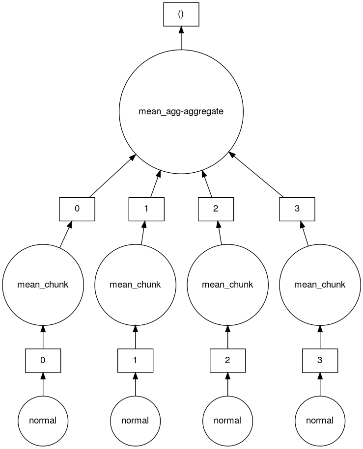
Here you can see that there are 4 tasks which create 4 array chunks from the normal distribution. These chunks are then input to the mean function which calculates the mean on each chunk. Finally a mean function which aggregates all the means of the chunks together is called to produce the final result.

Array distributed

These arrays are getting kind of big and processing them either in parallel or in serial on a single compute node restricts us to nodes that have more than about 7G of memory. Now on real clusters 7G of memory isn’t too bad but if arrays get bigger this could easily start to restrict how many of the nodes on the clusters you can run your jobs on to only the fewer more expensive large memory nodes. However, Dask is already processing our arrays in separate chunks on the same node couldn’t we distributed it across multiple nodes and reduce our memory requirement for an individual node?

If we wanted to be able to run on computations of large arrays with less memory per compute node could we distributed these computations across multiple nodes? Yes we can using the distributed computing method we saw earlier.
Solution

Start with the array-mean.py script we just created and add to it the distributed Dask cluster creation code.
$ cp array-mean.py array-distributed-mean.py
$ nano array-distributed-mean.py
import time
import dask.array as da
from dask_jobqueue import SLURMCluster
from dask.distributed import Client
...
def main():
...
  #memory=6G data / 16chunks x 4 cores per worker =1.5G plus a little extra
  cluster=SLURMCluster(cores=1,memory="2G",walltime='00:05:00')
  client=Client(cluster)
  cluster.scale(numWorkers)
  time.sleep(5)

  start=time.time()
  mean=meanDelayed.compute()
  computeTime=elapsed(start)

  client.close()
  cluster.close()
...
array-distributed-mean.py
$ srun python array-distributed-mean.py&
$ sqcm
  JOBID PARTITION     NAME   USER ST  TIME NODES CPUS MIN_M NODELIST
   1748 cpubase_b   python user49  R  0:05     1    1  256M node-sml1
   1749 cpubase_b dask-wor user49  R  0:01     1    1    2G node-sml1
   1750 cpubase_b dask-wor user49  R  0:01     1    1    2G node-sml2
   1751 cpubase_b dask-wor user49  R  0:01     1    1    2G node-mdm1
   1752 cpubase_b dask-wor user49  R  0:01     1    1    2G node-mdm1
Each of our workers is only using 2G of memory. While overall we are using 8G+256M of memory each compute node only has to have 2G of memory available, not the whole 7G on a single node that we needed for the serial or multi-threaded processing we did previously.
mean is -1.0935938328889444e-06

==================================
compute time: 9.609684467315674s
==================================


----------------------------------------
wall clock time:16.987823486328125s
----------------------------------------
It took a little longer to do the computation than it did when the computing happened all on the same node and there was extra time to create the cluster and wait for it to spin up, but it did allow us to do our computation with less memory per node and that can be very valuable in getting your job through the work queue faster on a production system as large memory nodes are few and very sought after.

Key Points

Wrapping Up

Overview

Teaching: 5 min
Exercises: min

Questions

What did we learn?

What next?

Objectives

Summary

Dask uses dask.delayed to compute task graphs.
These task graphs can then be later used to compute the result in either a multi-threaded or distributed way.
Multi-threaded python only benefits from the parallelism if it does considerable work outside the Python interpreter because of the GIL (e.g. NumPy etc.).
Distributed parallel Python code works well for most Python code but has a bit of an extra overhead for message-passing, start up/tear down of Dask cluster.
Python code is slow, but Cython can be used to easily compile computationally intensive parts into faster C code.
Dask Array provides a way to parallelize NumPy arrays either in a multi-threaded way for faster computing, or in a distributed way to reduce the individual compute node memory requirements and still give a reasonable speed up over serial execution.

Futher reading

On topics we have covered there can be more to learn. Check out these docs.

There are also some main features of Dask we didn’t talk about.

Dask DataFrames which provide a Pandas like interface. See also Data Frames best practices.
Dask Bag which implements operations like, map,filter, fold, and groupby on collections of generic Python objects similar to PyToolz or a Pythonic version of PySpark.
Dask Futures which supports a real-time task framework, similar to dask.delayed but is immediate rather than lazy.

Key Points

ACENET Summer School - Dask

Introduction

Overview

Dask tries to be familiar

How does Dask work?

Dask creates task graphs

Dask schedules tasks

Beginnings of Dask

Key Points

Python

Overview

Virtual environment setup

Running a Python script

Timing

Running on a compute node

A more interesting script

Key Points

Dask Delayed

Overview

Installing Dask

Using Dask Delayed

Parallelize a loop

Solution

Serial

Delayed Serial

Delayed 2 CPUs

Delayed 4 CPUs

Visualize loop parallelization

Solution

Parallelize loop with flow control

Solution

Key Points

Break

Overview

Key Points

Real Computations

Overview

More cores!

Solution

1 core

2 cores

4 cores

CPU efficiency

Solution

1 core

2 cores

4 cores

Key Points

Lunch Break

Overview

Key Points

Distributed Computations

Overview

More cores distributed

Solution

numWorkers=1

numWorkers=2

numWorkers=4

numWorkers=8

Running on busy clusters

Key Points

Cython

Overview

Cythonize our compute-distributed.py script

Solution

Key Points

NumPy

Overview

NumPy array vs. Python lists

Solution

Key Points

Break

Overview

Key Points

Dask Array

Overview

Array distributed

Solution

Key Points

Wrapping Up